Contents

Analysis Examples 2

Compare with traditional Neural Spike Train Analysis here

% load the rat trajectory and spiking data;
close all;
warning off;
installPath = which('nSTAT_Install');
if isempty(installPath)
    error('AnalysisExamples2:MissingInstallPath', ...
        'Could not locate nSTAT_Install.m on the MATLAB path.');
end
glmDataPath = fullfile(fileparts(installPath), 'data', 'glm_data.mat');
load(glmDataPath);

nst = nspikeTrain(spiketimes);
baseline = Covariate(T,ones(length(xN),1),'Baseline','time','s','',{'mu'});
position = Covariate(T,[xN yN],'Position', 'time','s','m',{'x','y'});
velocity = Covariate(T,[vxN,vyN],'Velocity','time','s','m/s',{'v_x','v_y'});
radial   = Covariate(T,[xN yN xN.^2 yN.^2 xN.*yN],'Radial','time','s','m',{'x','y','x^2','y^2','x*y'});
% could just define velocity = postion.derivative;

%possibly add view as vector for covariates of dimension 3 or less

In the original analysis, we already had vectors of the covariates sampled at the spiketimes. This step would require interpolating the covariates and then sampling them at each of the spikeTimes. In our case this is quite simple.

[values_at_spiketimes] =position.getValueAt(spiketimes);

We could also upsample our data to get better estimates of the covariates at these points

[values_at_spiketimes] =position.resample(1/min(diff(spiketimes))).getValueAt(spiketimes);

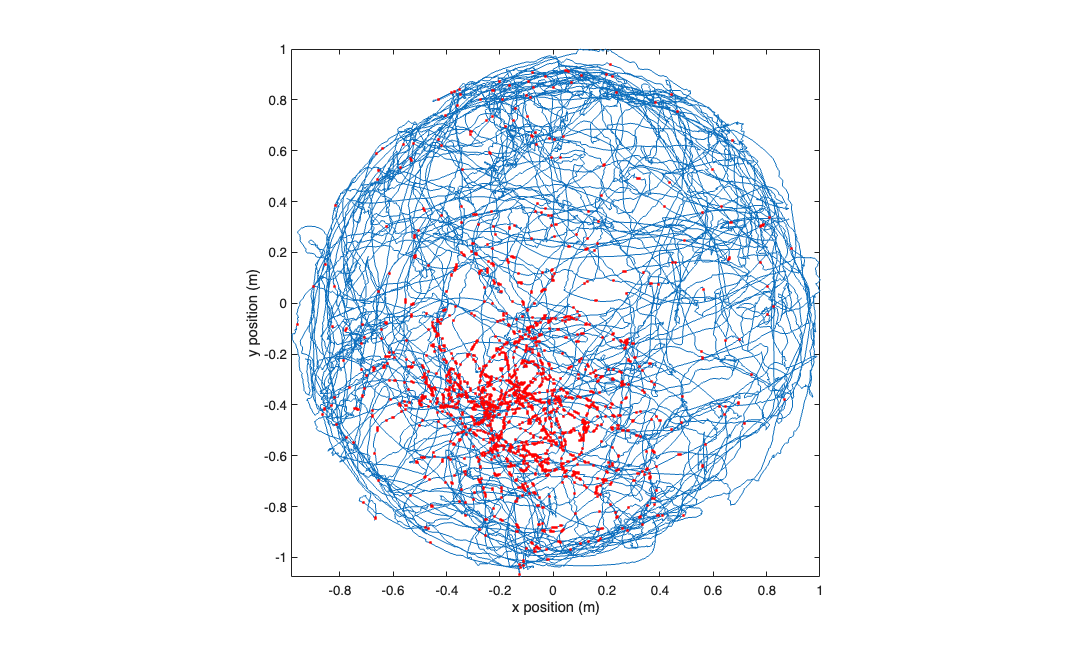
visualize the raw data

figure;
plot(position.getSubSignal('x').dataToMatrix,position.getSubSignal('y').dataToMatrix,...
     values_at_spiketimes(:,1),values_at_spiketimes(:,2),'r.');
axis tight square;
xlabel('x position (m)'); ylabel('y position (m)');

Create a trial object and define the fits that we want to run

spikeColl = nstColl({nst});
covarColl = CovColl({baseline,radial});
trial     = Trial(spikeColl,covarColl);
clear tc;
sampleRate=1000;
% tcObj=TrialConfig(covMask,sampleRate, history,minTime,maxTime)
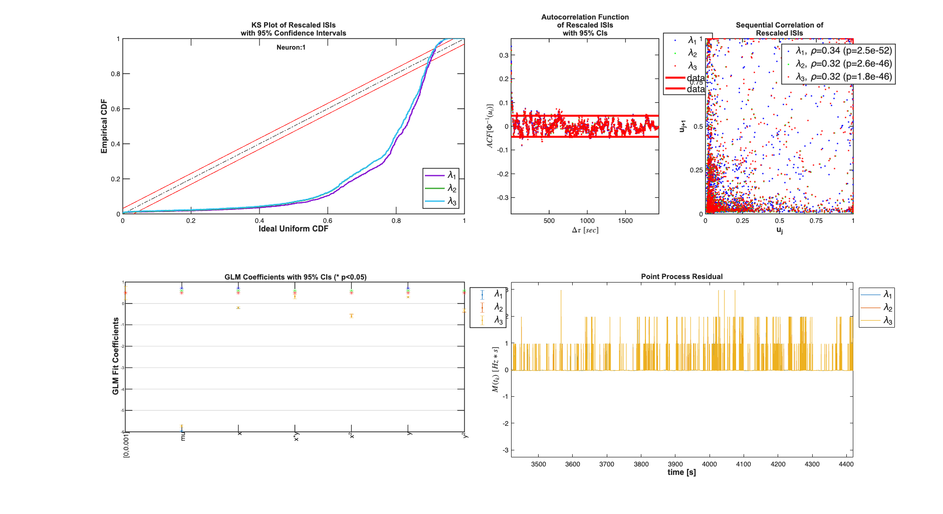
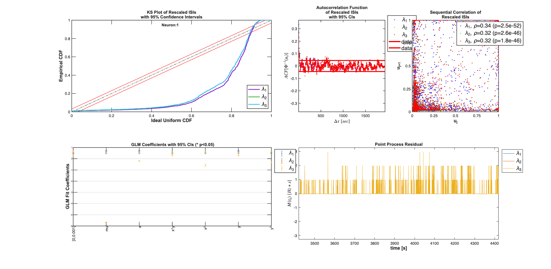
tc{1} = TrialConfig({{'Baseline','mu'},{'Radial','x','y'}},sampleRate,[]); tc{1}.setName('Linear');
tc{2} = TrialConfig({{'Baseline','mu'},{'Radial','x','y','x^2','y^2','x*y'}},sampleRate,[]); tc{2}.setName('Quadratic');
tc{3} = TrialConfig({{'Baseline','mu'},{'Radial','x','y','x^2','y^2','x*y'}},sampleRate,[0 1]./sampleRate); tc{3}.setName('Quadratic+Hist');

Create our collection of configurations and run the analysis;

tcc = ConfigColl(tc); makePlot=1; neuronNum=1;
fitResults =Analysis.RunAnalysisForAllNeurons(trial,tcc,0);
fitResults.plotResults;

Analyzing Configuration #1: Neuron #1
Analyzing Configuration #2: Neuron #1
Analyzing Configuration #3: Neuron #1

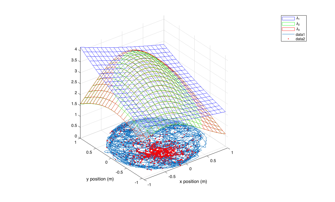
Visualize the firing rates as a function of the spatial covariates

figure;
[x_new,y_new]=meshgrid(-1:.1:1); %define new x and y
y_new = flipud(y_new);
x_new = fliplr(x_new);

%For each covariate new to place the new data in a cell array
newData{1} =ones(size(x_new));
newData{2} =x_new; newData{3} =y_new;
newData{4} =x_new.^2; newData{5} =y_new.^2;
newData{6} =x_new.*y_new;
color = Analysis.colors;

% Evaluate our fits using the new parameters
for i=1:fitResults.numResults

    lambda = fitResults.evalLambda(i,newData);
    h_mesh = mesh(x_new,y_new,lambda,'AlphaData',0);
    get(h_mesh,'AlphaData');
    set(h_mesh,'FaceAlpha',0.2,'EdgeAlpha',0.8,'EdgeColor',color{i});
    %figure;
    hold on;
end
legend(fitResults.lambda.dataLabels);
plot(position.getSubSignal('x').dataToMatrix,position.getSubSignal('y').dataToMatrix,...
     values_at_spiketimes(:,1),values_at_spiketimes(:,2),'r.');
axis tight square;
xlabel('x position (m)'); ylabel('y position (m)');

Toolbox vs. Standard GLM comparison

Compare the results using our approach with the standard approach used in the first example previous standard regression

[b,dev,stats] = glmfit([xN yN xN.^2 yN.^2 xN.*yN],spikes_binned,'poisson');
b-fitResults.b{2} % should be close to zero

ans =

    4.2365
   -1.4577
   -3.2263
   -6.3420
   -4.1806
   -0.3615

Compute the history effect

sampleRate=1000;  makePlot=1; neuronNum = 1;
covLabels = {{'Baseline','mu'},{'Radial','x','y','x^2','y^2','x*y'}};
Algorithm = 'GLM';
batchMode=0;
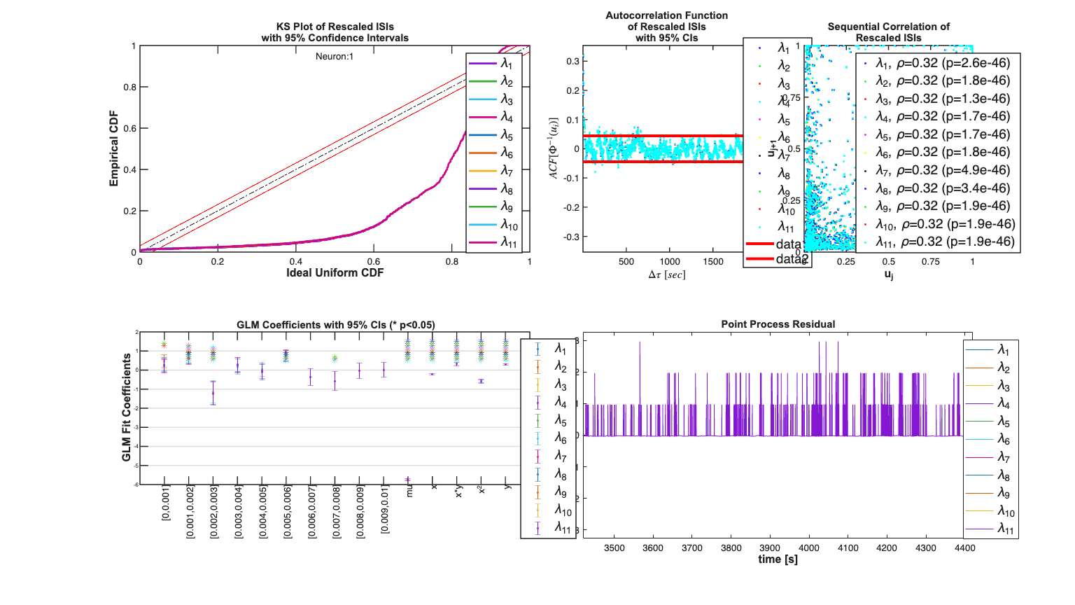
windowTimes =(0:1:10)./sampleRate;
% [fitResults,tcc] = computeHistLag(tObj,neuronNum,windowTimes,CovLabels,Algorithm,batchMode,sampleRate,makePlot,histMinTimes,histMaxTimes)
[fitResults,tcc] = Analysis.computeHistLag(trial,neuronNum,windowTimes,covLabels,Algorithm,batchMode,sampleRate,makePlot);

Analyzing Configuration #1: Neuron #1
Analyzing Configuration #2: Neuron #1
Analyzing Configuration #3: Neuron #1
Analyzing Configuration #4: Neuron #1
Analyzing Configuration #5: Neuron #1
Analyzing Configuration #6: Neuron #1
Analyzing Configuration #7: Neuron #1
Analyzing Configuration #8: Neuron #1
Analyzing Configuration #9: Neuron #1
Analyzing Configuration #10: Neuron #1
Analyzing Configuration #11: Neuron #1

Published with MATLAB® R2025b