EXPLICIT STIMULUS EXAMPLE - WHISKER STIMULATION/THALAMIC NEURON

In the worksheet with analyze the stimulus effect and history effect on the firing of a thalamic neuron under a known stimulus consisting of whisker stimulation. Data from Demba Ba (demba@mit.edu)

Load the data
Fit a constant baseline and Find Stimulus Lag
Compare constant rate model with model including stimulus effect
History Effect
Compare Baseline, Baseline+Stimulus Model, Baseline+History+Stimulus

Load the data

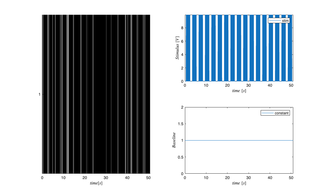
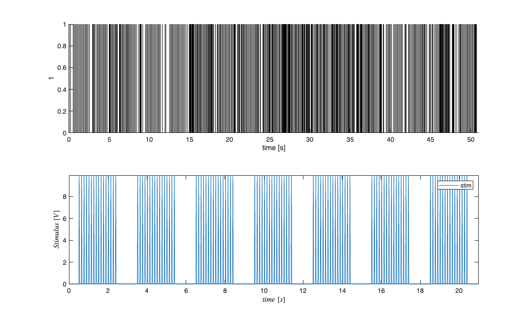
close all;
[~,~,explicitStimulusDir] = getPaperDataDirs();

Direction=3; Neuron=1; Stim=2;
datapath = fullfile(explicitStimulusDir,strcat('Dir', num2str(Direction)),...
    strcat('Neuron', num2str(Neuron)), strcat('Stim', num2str(Stim)));
data=load(fullfile(datapath,'trngdataBis.mat'));

time=0:.001:(length(data.t)-1)*.001;
stimData = data.t;
spikeTimes = time(data.y==1);

stim = Covariate(time,stimData,'Stimulus','time','s','V',{'stim'});
baseline = Covariate(time,ones(length(time),1),'Baseline','time','s','',...
    {'constant'});

nst = nspikeTrain(spikeTimes);
nspikeColl = nstColl(nst);
cc = CovColl({stim,baseline});
trial = Trial(nspikeColl,cc);
trial.plot;

figure;
subplot(2,1,1);
nst2 = nspikeTrain(spikeTimes);
nst2.setMaxTime(21);nst.plot;
subplot(2,1,2);
stim.getSigInTimeWindow(0,21).plot;

Fit a constant baseline and Find Stimulus Lag

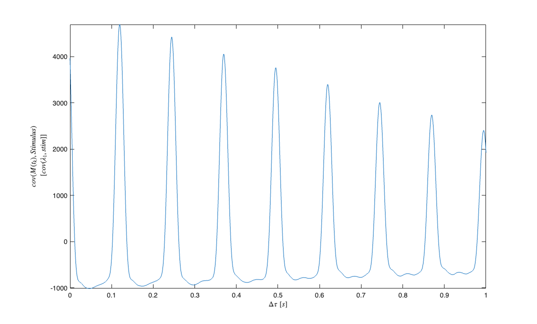
We fit a constant rate (Poisson) model to the data and use the fit residual to determine the appropriate lag for the stimulus.

clear c;
selfHist = [] ; NeighborHist = []; sampleRate = 1000;
c{1} = TrialConfig({{'Baseline','constant'}},sampleRate,selfHist,NeighborHist);
c{1}.setName('Baseline');
cfgColl= ConfigColl(c);
results = Analysis.RunAnalysisForAllNeurons(trial,cfgColl,0);

% Find Stimulus Lag (look for peaks in the cross-covariance function less
% than 1 second
figure;
results.Residual.xcov(stim).windowedSignal([0,1]).plot;
[m,ind,ShiftTime] = max(results.Residual.xcov(stim).windowedSignal([0,1]));
%Allow for shifts of less than 1 second
stim = Covariate(time,stimData,'Stimulus','time','s','V',{'stim'});
stim = stim.shift(ShiftTime);
baseline = Covariate(time,ones(length(time),1),'Baseline','time','s','',...
    {'constant'});

nst = nspikeTrain(spikeTimes);
nspikeColl = nstColl(nst);
cc = CovColl({stim,baseline});
trial = Trial(nspikeColl,cc);

Analyzing Configuration #1: Neuron #1

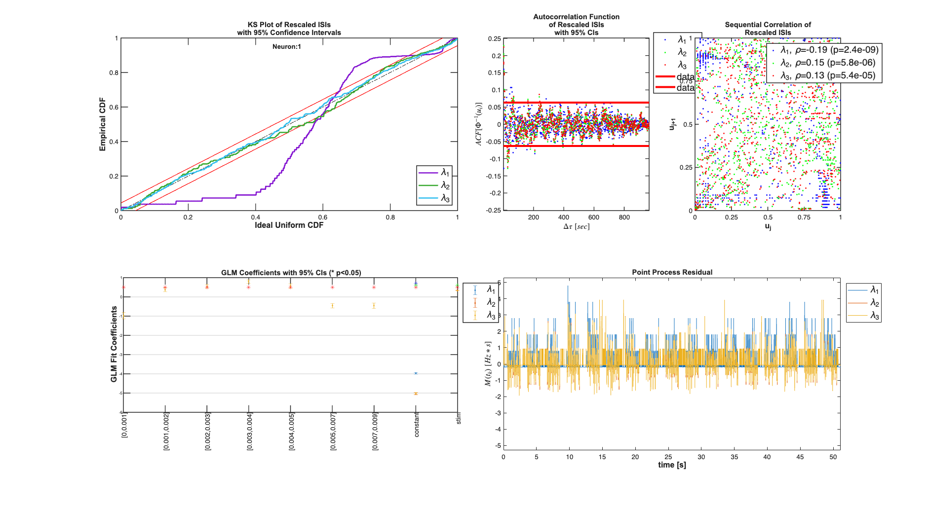
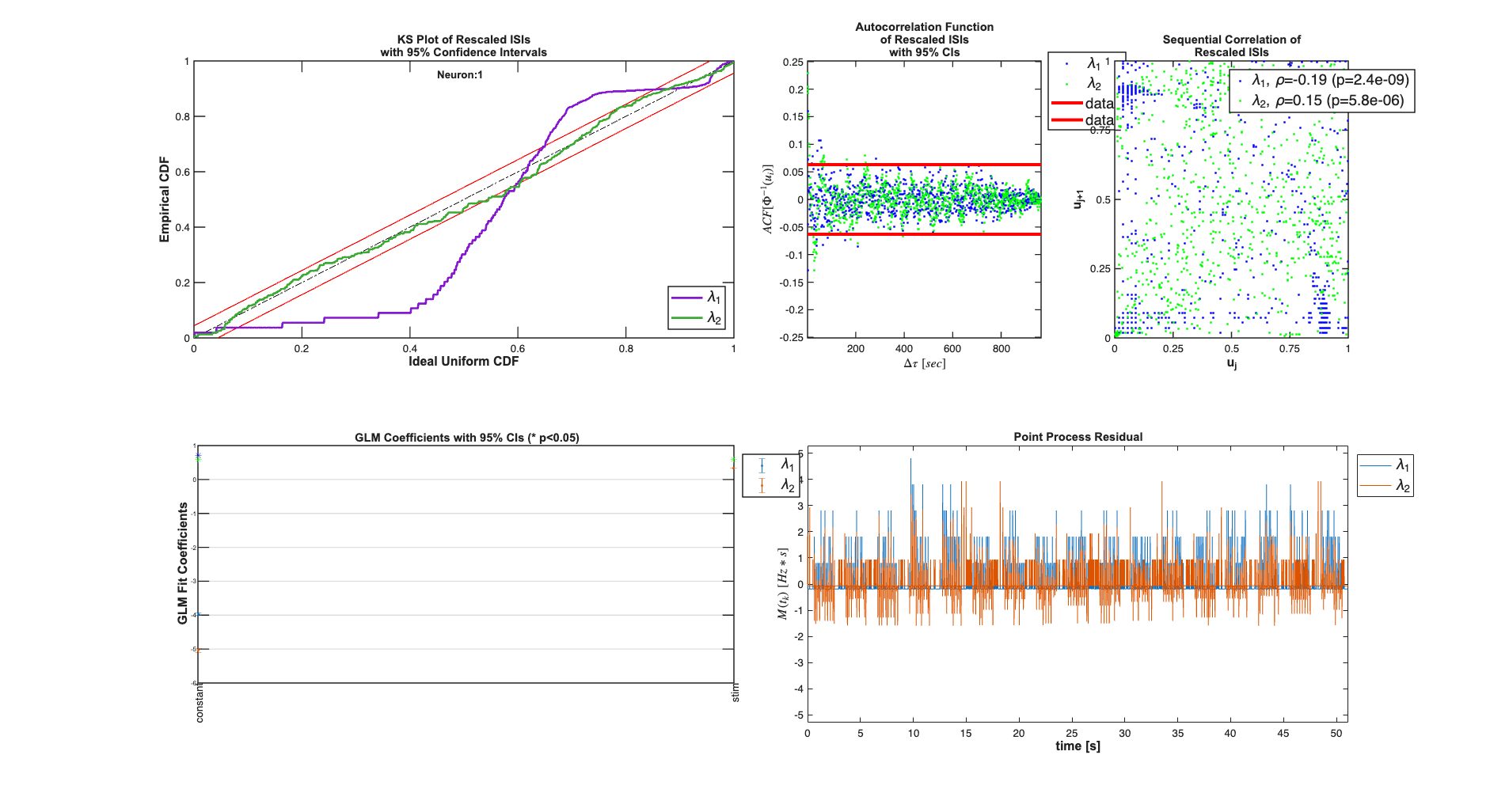
Compare constant rate model with model including stimulus effect

Addition of the stimulus improves the fits in terms of the KS plot and the making the rescaled ISIs less correlated. The Point Process Residula also looks more "white"

clear c;
selfHist = [] ; NeighborHist = []; sampleRate = 1000;
c{1} = TrialConfig({{'Baseline','constant'}},sampleRate,selfHist,...
    NeighborHist);
c{1}.setName('Baseline');
c{2} = TrialConfig({{'Baseline','constant'},{'Stimulus','stim'}},...
    sampleRate,selfHist,NeighborHist);
c{2}.setName('Baseline+Stimulus');
cfgColl= ConfigColl(c);
results = Analysis.RunAnalysisForAllNeurons(trial,cfgColl,0);
results.plotResults;

Analyzing Configuration #1: Neuron #1
Analyzing Configuration #2: Neuron #1

History Effect

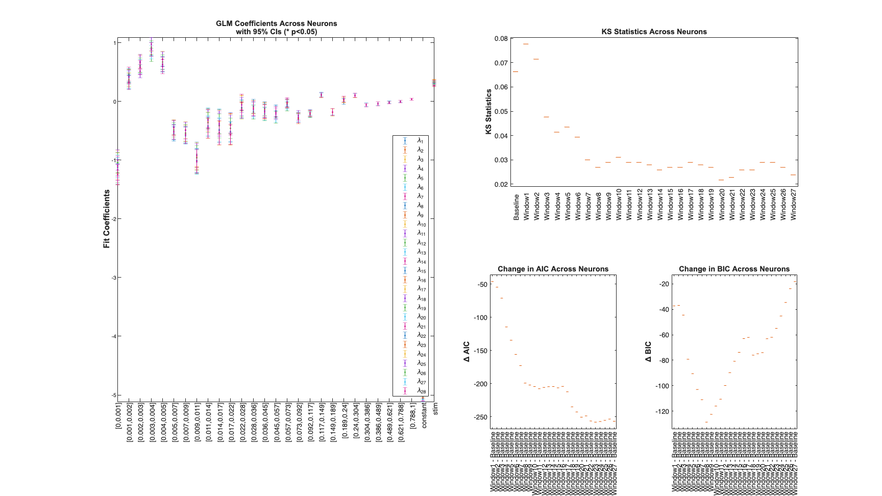
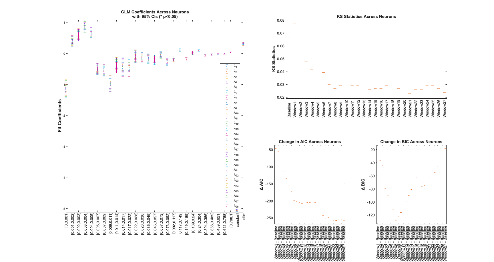
Determine the best history effect model using AIC, BIC, and KS statistic

sampleRate=1000;
delta=1/sampleRate*1;
maxWindow=1; numWindows=30;
windowTimes =unique(round([0 logspace(log10(delta),...
    log10(maxWindow),numWindows)]*sampleRate)./sampleRate);
results =Analysis.computeHistLagForAll(trial,windowTimes,...
    {{'Baseline','constant'},{'Stimulus','stim'}},'BNLRCG',0,sampleRate,0);

KSind = find(results{1}.KSStats.ks_stat == min(results{1}.KSStats.ks_stat));
AICind = find((results{1}.AIC(2:end)-results{1}.AIC(1))== ...
               min(results{1}.AIC(2:end)-results{1}.AIC(1)));
BICind = find((results{1}.BIC(2:end)-results{1}.BIC(1))== ...
               min(results{1}.BIC(2:end)-results{1}.BIC(1)));
if(AICind==1)
    AICind=inf;
end
if(BICind==1)
    BICind=inf; %sometime BIC is non-decreasing and the index would be 1
end
windowIndex = min([KSind,AICind,BICind]) %use the minimum order model
Summary = FitResSummary(results);
Summary.plotSummary;


clear c;
if(windowIndex>1)
    selfHist = windowTimes(1:windowIndex);
else
    selfHist = [];
end
NeighborHist = []; sampleRate = 1000;

Analyzing Configuration #1: Neuron #1
Analyzing Configuration #2: Neuron #1
Analyzing Configuration #3: Neuron #1
Analyzing Configuration #4: Neuron #1
Analyzing Configuration #5: Neuron #1
Analyzing Configuration #6: Neuron #1
Analyzing Configuration #7: Neuron #1
Analyzing Configuration #8: Neuron #1
Analyzing Configuration #9: Neuron #1
Analyzing Configuration #10: Neuron #1
Analyzing Configuration #11: Neuron #1
Analyzing Configuration #12: Neuron #1
Analyzing Configuration #13: Neuron #1
Analyzing Configuration #14: Neuron #1
Analyzing Configuration #15: Neuron #1
Analyzing Configuration #16: Neuron #1
Analyzing Configuration #17: Neuron #1
Analyzing Configuration #18: Neuron #1
Analyzing Configuration #19: Neuron #1
Analyzing Configuration #20: Neuron #1
Analyzing Configuration #21: Neuron #1
Analyzing Configuration #22: Neuron #1
Analyzing Configuration #23: Neuron #1
Analyzing Configuration #24: Neuron #1
Analyzing Configuration #25: Neuron #1
Analyzing Configuration #26: Neuron #1
Analyzing Configuration #27: Neuron #1
Analyzing Configuration #28: Neuron #1

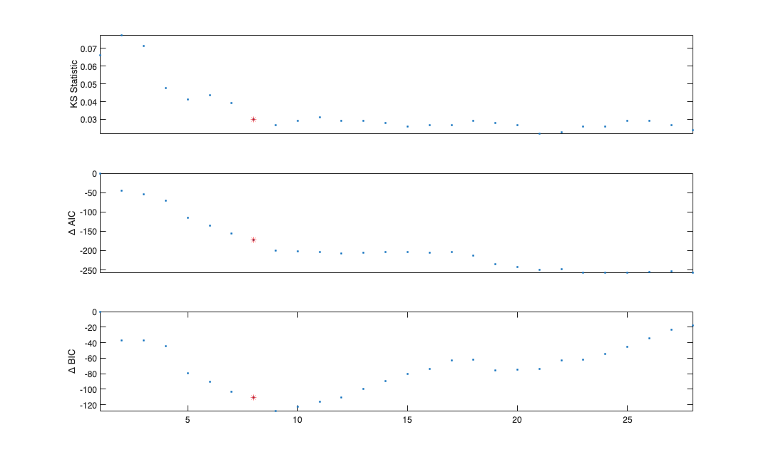
windowIndex =

     8

figure;
x=1:length(windowTimes);
subplot(3,1,1); plot(x,results{1}.KSStats.ks_stat,'.'); axis tight; hold on;
plot(x(windowIndex),results{1}.KSStats.ks_stat(windowIndex),'r*');

 set(gca,'xtick',[]);
ylabel('KS Statistic');
dAIC = results{1}.AIC-results{1}.AIC(1);
subplot(3,1,2); plot(x,dAIC,'.');
 set(gca,'xtick',[]);
ylabel('\Delta AIC');axis tight; hold on;
plot(x(windowIndex),dAIC(windowIndex),'r*');
dBIC = results{1}.BIC-results{1}.BIC(1);
subplot(3,1,3); plot(x,dBIC,'.');
ylabel('\Delta BIC'); axis tight; hold on;
plot(x(windowIndex),dBIC(windowIndex),'r*');

for i=2:length(x)
   histLabels{i} = ['[' num2str(windowTimes(i-1),3) ',' num2str(windowTimes(i),3) ,']'];
end

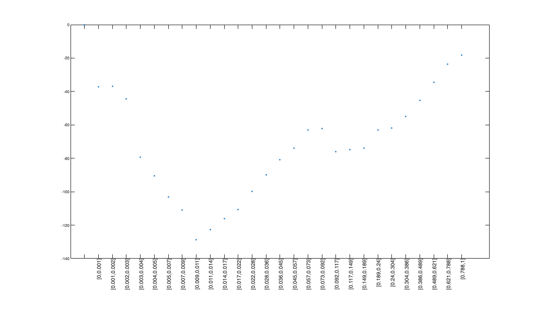
figure;
plot(x,dBIC,'.');
xticks = 1:(length(histLabels));
set(gca,'xtick',xticks,'xtickLabel',histLabels,'FontSize',6);
if(max(xticks)>=1)
    xticklabel_rotate([],90,[],'Fontsize',8);
end

Compare Baseline, Baseline+Stimulus Model, Baseline+History+Stimulus

Addition of the history effect yields a model that falls within the 95% CI of the KS plot.

c{1} = TrialConfig({{'Baseline','constant'}},sampleRate,[],NeighborHist);
c{1}.setName('Baseline');
c{2} = TrialConfig({{'Baseline','constant'},{'Stimulus','stim'}},...
                    sampleRate,[],[]);
c{2}.setName('Baseline+Stimulus');
c{3} = TrialConfig({{'Baseline','constant'},{'Stimulus','stim'}},...
                    sampleRate,windowTimes(1:windowIndex),[]);
c{3}.setName('Baseline+Stimulus+Hist');
cfgColl= ConfigColl(c);
results = Analysis.RunAnalysisForAllNeurons(trial,cfgColl,0);
results.plotResults;