HIPPOCAMPAL PLACE CELL - RECEPTIVE FIELD ESTIMATION
Estimation of receptive fields of neurons is a very common data analysis problem in neuroscience. Here we use the nSTAT software to perform an estimation of the receptive fields of hippocampal place cells using a bivariate Gaussian model and Zernike polynomials. The number of zernike polynomials is based on "An Analysis of Hippocampal Spatio-Temporal Representations Using a Bayesian Algorithm for Neural Spike Train Decoding" Barbieri et. al 2005. The data used herein in was provided by Dr. Ricardo Barbieri on 2/28/2011.
Author: Iahn Cajigas
Date: 3/1/2011
Contents
close all
[~,~,~,~,placeCellDataDir] = getPaperDataDirs();
Example Data
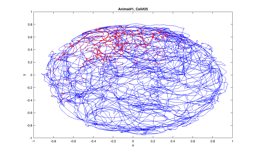
The x and y coordinates of a freely foraging rat in a circular environment (70cm in diameter and 30cm high walls) and a fixed visual cue. The x and y coordinates at the time when a spike was observed are marked in red. The position coordinates have been normalized to be between -1 and 1 to allow to simplify the analysis.
    load(fullfile(placeCellDataDir,'PlaceCellDataAnimal1.mat'));
    exampleCell = 25;
    figure(1);
    plot(x,y,'b',neuron{exampleCell}.xN,neuron{exampleCell}.yN,'r.');
    xlabel('x'); ylabel('y');
    title(['Animal#1, Cell#' num2str(exampleCell)]);
Analyze All Cells
 numAnimals =2;
for n=1:numAnimals
    % load the data
    clear x y neuron time nst tc tcc z;
    load(fullfile(placeCellDataDir,['PlaceCellDataAnimal' num2str(n) '.mat']));

    % Create the spikeTrains for each cell
    for i=1:length(neuron)
        nst{i} = nspikeTrain(neuron{i}.spikeTimes);
    end


    % Convert to polar coordinates
    [theta,r] = cart2pol(x,y);


    % Evaluate the Zernike Polynomials
    % Number of polynomials from "An Analysis of Hippocampal
    % Spatio-Temporal Representations Using a Bayesian Algorithm for Neural
    % Spike Train Decoding" Barbieri et. al 2005
    cnt=0;
    for l=0:3
       for m=-l:l
           if(~any(mod(l-m,2))) % otherwise the polynomial = 0
            cnt = cnt+1;
            z(:,cnt) = zernfun(l,m,r,theta,'norm');
            % zernfun by Paul Fricker
            % http://www.mathworks.com/matlabcentral/fileexchange/7687
           end
       end
    end

    % Data sampled at 30 Hz but just to be sure
    delta=min(diff(time));
    sampleRate = round(1/delta);

    % Define Covariates for the analysis
    baseline = Covariate(time,ones(length(x),1),'Baseline','time','s','',...
                        {'mu'});
    zernike  = Covariate(time,z,'Zernike','time','s','m',{'z1','z2','z3',...
                        'z4','z5','z6','z7','z8','z9','z10'});
    gaussian = Covariate(time,[x y x.^2 y.^2 x.*y],'Gaussian','time',...
                        's','m',{'x','y','x^2','y^2','x*y'});
    covarColl = CovColl({baseline,gaussian,zernike});

    % Create the trial structure
    spikeColl = nstColl(nst);
    trial     = Trial(spikeColl,covarColl);


    % Define how we want to analyze the data
    tc{1} = TrialConfig({{'Baseline','mu'},{'Gaussian',...
                        'x','y','x^2','y^2','x*y'}},sampleRate,[]);
    tc{1}.setName('Gaussian');
    tc{2} = TrialConfig({{'Zernike' 'z1','z2','z3','z4','z5','z6',...
                        'z7','z8','z9','z10'}},sampleRate,[]);
    tc{2}.setName('Zernike');
    tcc = ConfigColl(tc);

    % Perform Analysis (Commented to since data already saved)
%     results =Analysis.RunAnalysisForAllNeurons(trial,tcc,0);

    % Save results
%     resStruct =FitResult.CellArrayToStructure(results);
%     filename = ['PlaceCellAnimal' num2str(n) 'Results'];
%     save(filename,'resStruct');
end
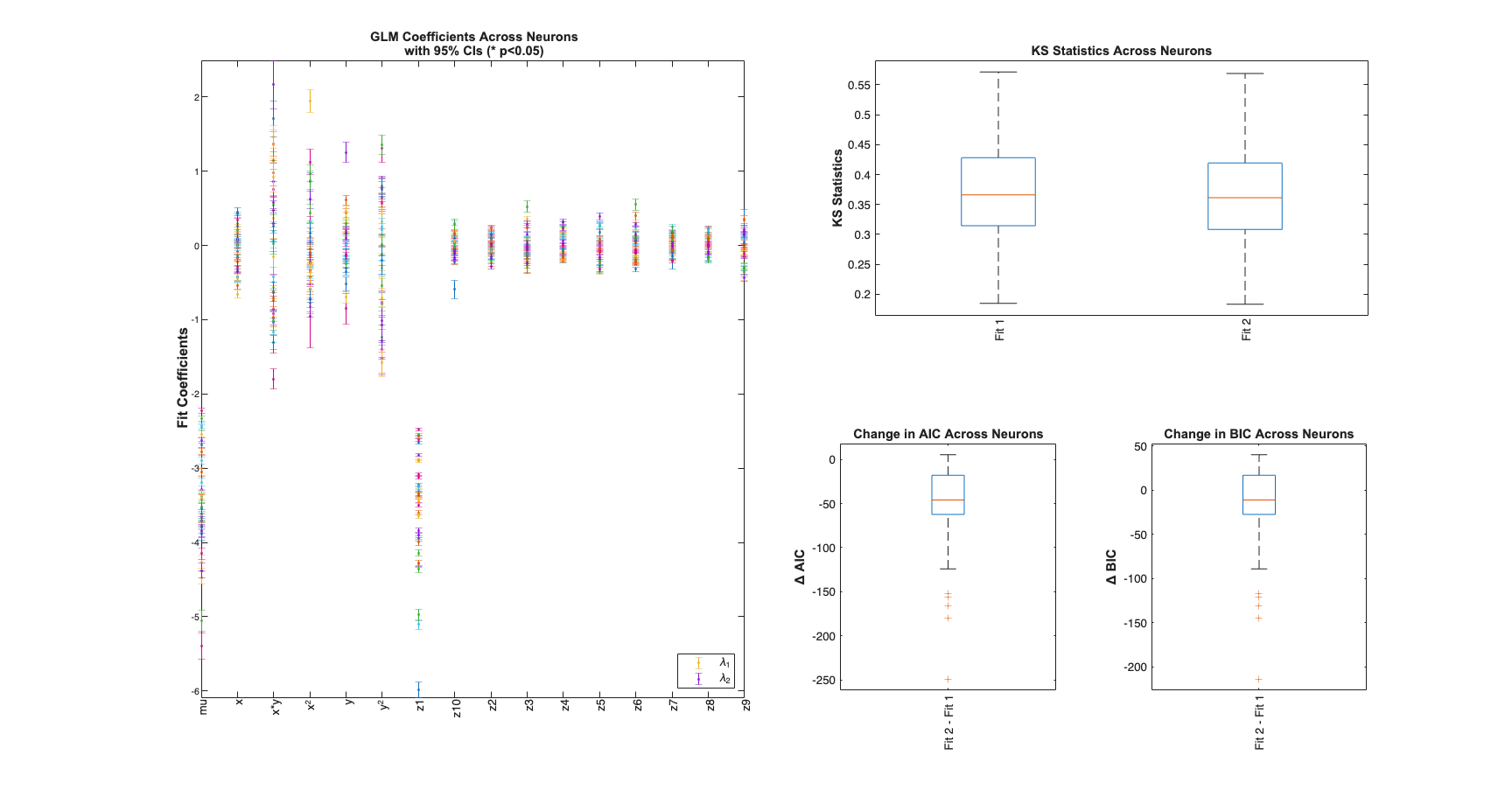
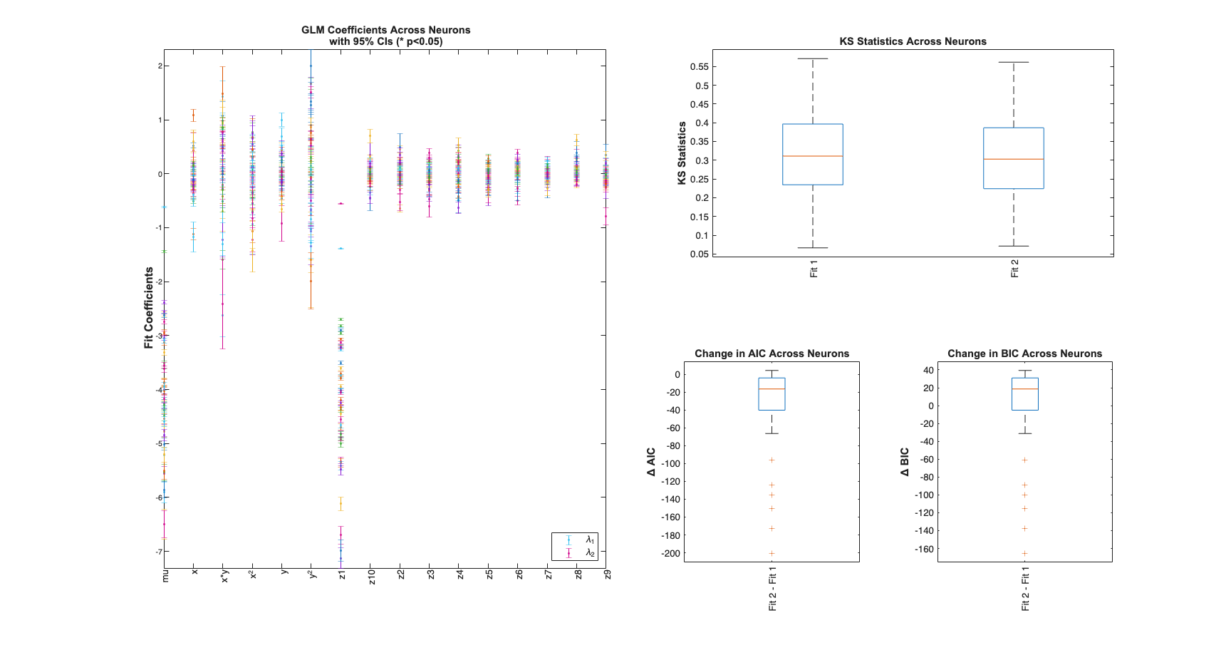
View Summary Statistics
Note the Zernike Polynomials yield better fits in terms of decreased KS Statistics (less deviation from the 45 degree line), reduced AIC and reduced BIC across the majority of cells and for both animals
for n=1:numAnimals
    resData=load(fullfile(fileparts(placeCellDataDir),['PlaceCellAnimal' num2str(n) 'Results.mat']));
    results = FitResult.fromStructure(resData.resStruct);
    Summary = FitResSummary(results);
    Summary.plotSummary;
end

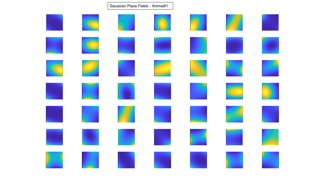
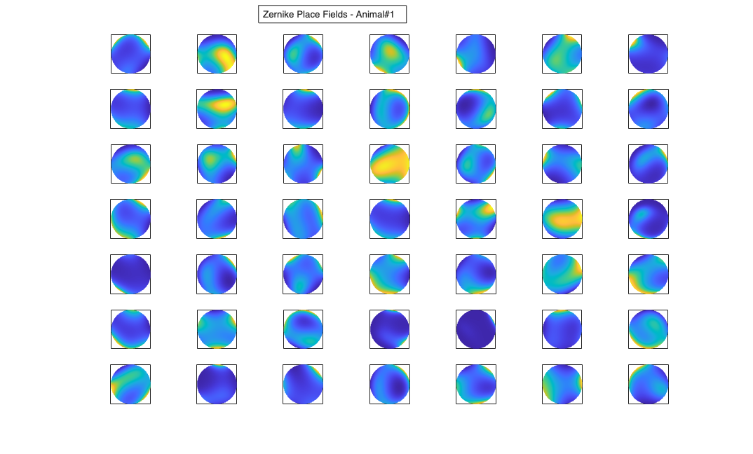
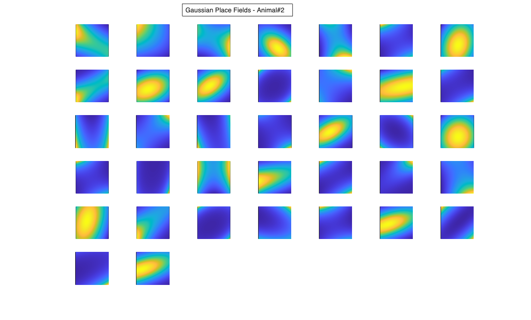
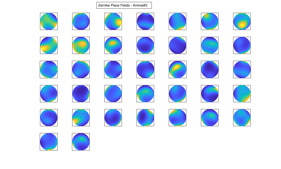
Visualize the results
% Define a grid
[x_new,y_new]=meshgrid(-1:.01:1); %define new x and y
y_new = flipud(y_new); x_new = fliplr(x_new);
[theta_new,r_new] = cart2pol(x_new,y_new);

%Data for the gaussian fit
newData{1} =ones(size(x_new));
newData{2} =x_new; newData{3} =y_new;
newData{4} =x_new.^2; newData{5} =y_new.^2;
newData{6} =x_new.*y_new;


% Zernike polynomials only defined on the unit disk
idx = r_new<=1;
zpoly = cell(1,10);
cnt=0;
for l=0:3
   for m=-l:l
       if(~any(mod(l-m,2)))
        cnt = cnt+1;
        temp = nan(size(x_new));
        temp(idx) = zernfun(l,m,r_new(idx),theta_new(idx),'norm');
        zpoly{cnt} = temp;
       end
   end
end


for n=1:numAnimals

    clear lambdaGaussian lambdaZernike;
    load(fullfile(placeCellDataDir,['PlaceCellDataAnimal' num2str(n) '.mat']));
    resData=load(fullfile(fileparts(placeCellDataDir),['PlaceCellAnimal' num2str(n) 'Results.mat']));
    results = FitResult.fromStructure(resData.resStruct);

    for i=1:length(neuron)
        % Evaluate our fits using the new data and the estimated parameters
        lambdaGaussian{i} = results{i}.evalLambda(1,newData);
        lambdaZernike{i} =  results{i}.evalLambda(2,zpoly);
    end


    % Plot the receptive fields
    for i=1:length(neuron)
        % 3d plot of an example place field


        % 2d plot of all the cell's fields
        if(n==1)
            h4=figure(4);
            if(i==1)
                annotation(h4,'textbox',...
                    [0.343261904761904 0.928571428571418 ...
                    0.392857142857143 0.0595238095238095],...
                    'String',{['Gaussian Place Fields - Animal#' ...
                    num2str(n)]},'FitBoxToText','on'); hold on;
            end
            subplot(7,7,i);
        elseif(n==2)
            h6=figure(6);
            if(i==1)
                annotation(h6,'textbox',...
                    [0.343261904761904 0.928571428571418 ...
                    0.392857142857143 0.0595238095238095],...
                    'String',{['Gaussian Place Fields - Animal#' ...
                    num2str(n)]},'FitBoxToText','on'); hold on;
            end
            subplot(6,7,i);
        end
        pcolor(x_new,y_new,lambdaGaussian{i}), shading interp
        axis square; set(gca,'xtick',[],'ytick',[]);


        if(n==1)
            h5=figure(5);
            if(i==1)
                annotation(h5,'textbox',...
                    [0.343261904761904 0.928571428571418 ...
                    0.392857142857143 0.0595238095238095],...
                    'String',{['Zernike Place Fields - Animal#' ...
                    num2str(n)]},'FitBoxToText','on'); hold on;

            end
            subplot(7,7,i);
        elseif(n==2)
            h7=figure(7);
            if(i==1)
               annotation(h7,'textbox',...
                    [0.343261904761904 0.928571428571418 ...
                    0.392857142857143 0.0595238095238095],...
                    'String',{['Zernike Place Fields - Animal#' ...
                    num2str(n)]},'FitBoxToText','on'); hold on;
            end
            subplot(6,7,i);
        end
        pcolor(x_new,y_new,lambdaZernike{i}), shading interp
        axis square;
        set(gca,'xtick',[],'ytick',[]);
    end


end


    clear lambdaGaussian lambdaZernike;
    load(fullfile(placeCellDataDir,'PlaceCellDataAnimal1.mat'));
    resData=load(fullfile(fileparts(placeCellDataDir),'PlaceCellAnimal1Results.mat'));
    results = FitResult.fromStructure(resData.resStruct);

    for i=1:length(neuron)
        % Evaluate our fits using the new data and the estimated parameters
        lambdaGaussian{i} = results{i}.evalLambda(1,newData);
        lambdaZernike{i} =  results{i}.evalLambda(2,zpoly);
    end


    exampleCell = 25;
    figure(8);
    plot(x,y,'b',neuron{exampleCell}.xN,neuron{exampleCell}.yN,'r.');
    xlabel('x'); ylabel('y');
    title(['Animal#1, Cell#' num2str(exampleCell)]);

    figure(9);
    h_mesh = mesh(x_new,y_new,lambdaGaussian{exampleCell},'AlphaData',0);
    get(h_mesh,'AlphaData');
    set(h_mesh,'FaceAlpha',0.2,'EdgeAlpha',0.2,'EdgeColor','b');
    hold on;
    h_mesh = mesh(x_new,y_new,lambdaZernike{exampleCell},'AlphaData',0);
    get(h_mesh,'AlphaData');
    set(h_mesh,'FaceAlpha',0.2,'EdgeAlpha',0.2,'EdgeColor','g');

    legend(results{exampleCell}.lambda.dataLabels);
    plot(x,y,neuron{exampleCell}.xN,neuron{exampleCell}.yN,'r.');
    axis tight square;
    xlabel('x position'); ylabel('y position');
    title(['Animal#1, Cell#' num2str(exampleCell)]);