General Point Process Simulation

In this demo, we show how sample-paths of a point process (PP) can be generated from specification of its conditional intensity function (CIF). We then use the generated PP data to validate the outputs of the Neural Spike Analysis Toolbox.

Contents

Point Process Sample Path Generation

That both the stimulus effect and ensemble effects can be made into multi-input/multi-output transfer functions to account for more than 1 stimulus effect or multiple neighboring neuron effects. To do this, simply define $E$ or $S$ to be a row vector of LTI transfer functions. Make sure than the number of dimensions of the input matches the number of transfer functions specified in the row vector.

Error in state of SceneNode.
String scalar or character vector must have valid interpreter syntax: 
$E$ or $

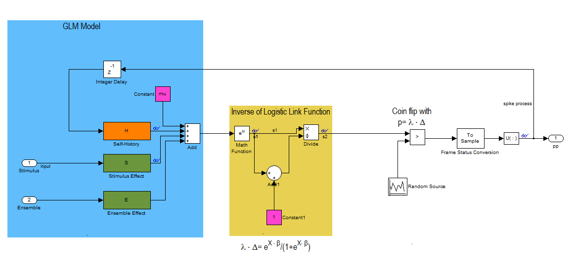
This block diagram specifies a conditional intensity function of the form

close all;
Ts=.001;            %Sample Time
tMin=0; tMax=50;    %Simulation duration
t=tMin:Ts:tMax;

mu=-3;              %Baseline firing rate of the neurons being modeled

History Effect

H=tf([-1 -2 -4],[1],Ts,'Variable','z^-1');

Stimulus Effect

S=tf([1],1,Ts,'Variable','z^-1');

Ensemble Effect

E=tf([0],1,Ts,'Variable','z^-1');

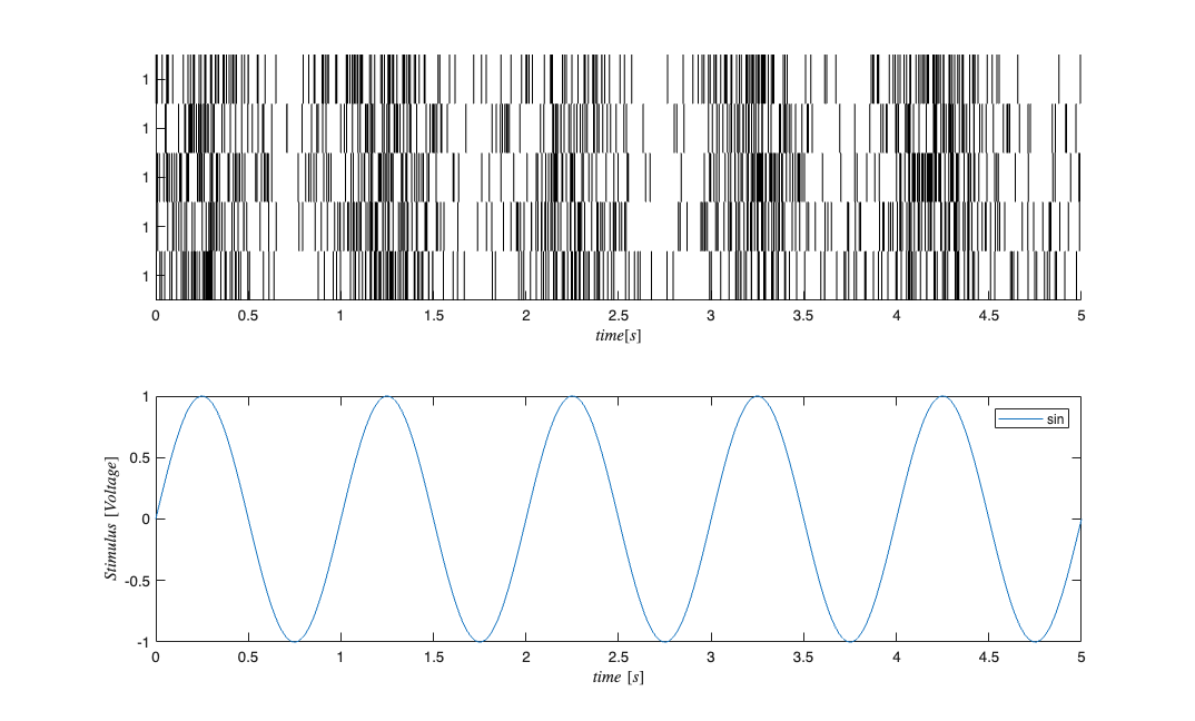
f=1;                    %Stimulus frequency
u = sin(2*pi*f*t)';       %Make this neuron modulated by a sine wave
e = zeros(length(t),1);   %No Ensemble input

stim=Covariate(t',u,'Stimulus','time','s','Voltage',{'sin'});
ens =Covariate(t',e,'Ensemble','time','s','Spikes',{'n1'});
numRealizations = 5;    %Number of sample paths to generate
fitType = 'binomial';
sC=CIF.simulateCIF(mu,H,S,E,stim,ens,numRealizations,fitType);
figure;
subplot(2,1,1); sC.plot;    v=axis; axis([0 tMax/10 v(3) v(4)]);
subplot(2,1,2); stim.plot;  v=axis; axis([0 tMax/10 v(3) v(4)]);

GLM Model Fitting Setup

In this section, we create the appropriate structures to fit several GLM models to the data generated above.

% Create a constant covariate representing the mean firing rate $$\mu_{i}$
baseline=Covariate(t',ones(length(t),1),'Baseline','time','s','',{'mu'});


spikeColl = sC;               %Use the generated data as our collection of spikes
cc=CovColl({stim,baseline});  %Use stimulation and baseline as possible covariates
trial = Trial(spikeColl,cc); sampleRate = 1/Ts; %Create trial

GLM Model Fitting and Results

clear c;
selfHist = [0:0.001:0.003]; %We know the history effect goes back 3 lag orders

Fit only a mean firing rate

c{1} = TrialConfig({{'Baseline','mu'}},sampleRate,[],[]);
c{1}.setName('Baseline');

Fit a mean firing rate + the stimulus term

c{2} = TrialConfig({{'Baseline','mu'},{'Stimulus','sin'}},sampleRate,[],[]);
c{2}.setName('Stim');

Fit a mean firing rate, self-history, and stimulus --- Same as true model

c{3} = TrialConfig({{'Baseline','mu'},{'Stimulus','sin'}},sampleRate,selfHist,[]);
c{3}.setName('Stim+Hist');

Place all configurations together and run analysis for each neuron

cfgColl= ConfigColl(c);
if(strcmp(fitType,'binomial'))
    Algorithm = 'BNLRCG';   % BNLRCG - faster Truncated, L-2 Regularized,
                            % Binomial Logistic Regression with Conjugate
                            % Gradient Solver by Demba Ba (demba@mit.edu).
else
    Algorithm = 'GLM';      % Standard Matlab GLM (Can be used for binomial or
                            % or Poisson CIFs
end
results = Analysis.RunAnalysisForAllNeurons(trial,cfgColl,0,Algorithm);

Analyzing Configuration #1: Neuron #1,2,3,4,5
Analyzing Configuration #2: Neuron #1,2,3,4,5
Analyzing Configuration #3: Neuron #1,2,3,4,5

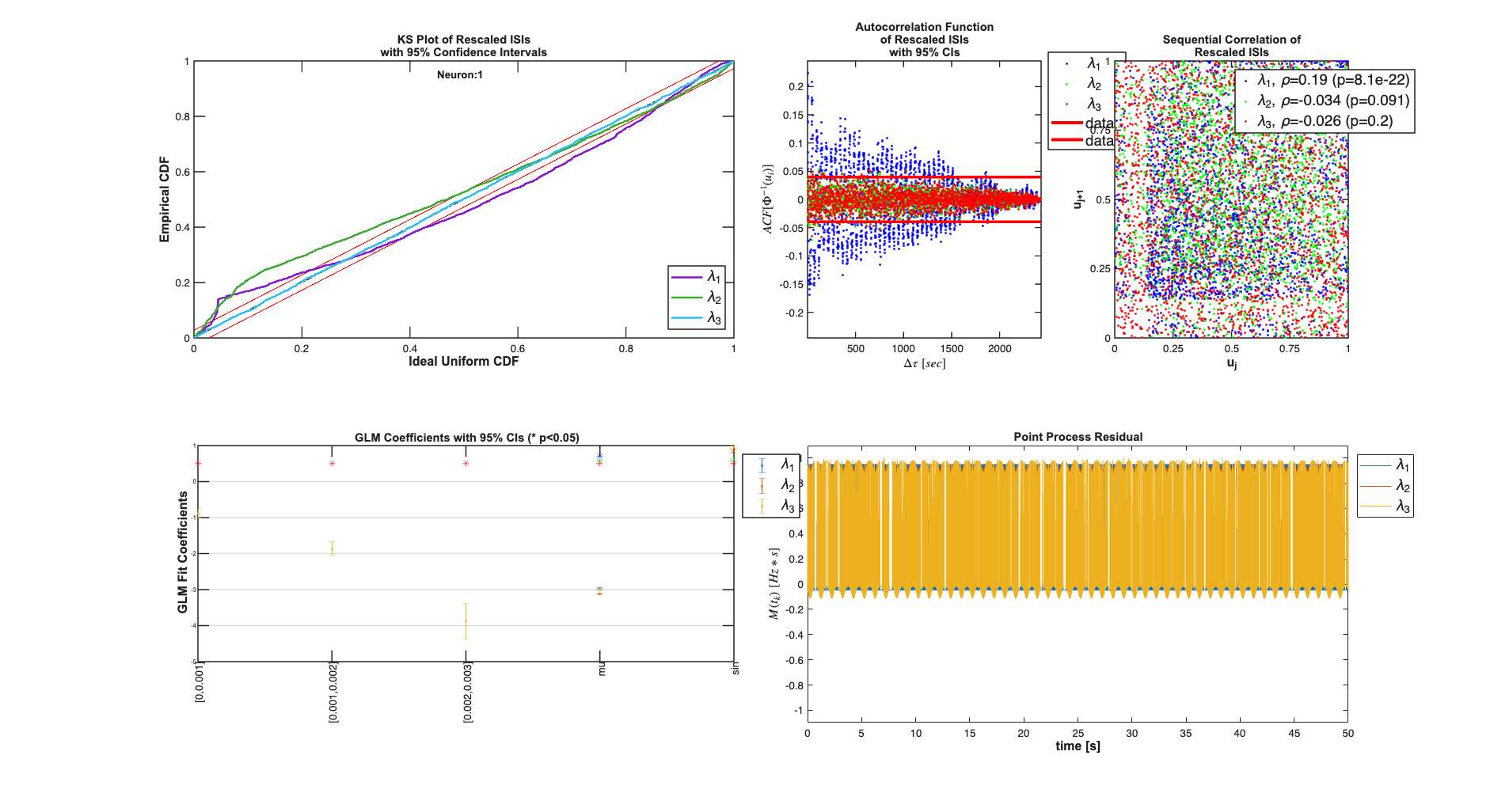
Results for sample neuron

results{1}.plotResults;

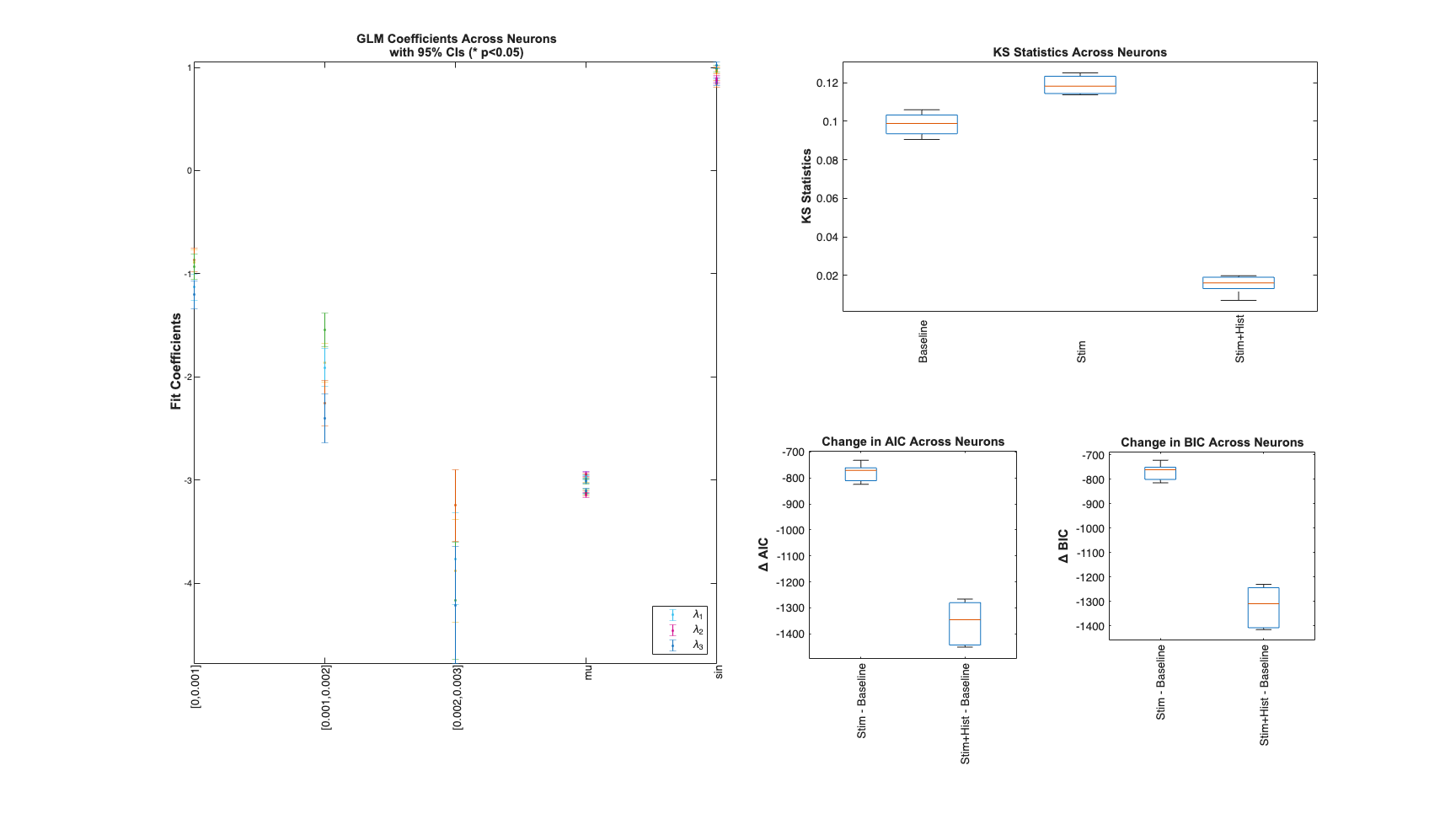
Results for across all sample paths

Summary = FitResSummary(results);
Summary.plotSummary;

Published with MATLAB® R2025b