Contents
- nSTAT J. Neuroscience Methods Paper Examples
- Experiment 1
- Constant Magnesium Concentration - Constant rate poisson
- Varying Magnesium Concentration - Piecewise Constant rate poisson
- Data Visualization
- Define Covariates for the analysis
- Define how we want to analyze the data
- Perform Analysis
- Experiment 2
- Load the data
- Compare constant rate model with model including stimulus effect
- History Effect
- Example 3 - PSTH Data
- Estimate the PSTH with 50ms windows
- Example 3b - SSGLM Example
- Summarize Simulated Data
- Estimation of the Stimulus Response
- Run the SSGLM Filter
- Compare differences across trials
- Example 4 - HIPPOCAMPAL PLACE CELL - RECEPTIVE FIELD ESTIMATION
- Example Data
- Analyze All Cells
- View Summary Statistics
- Visualize the results
- Example 5 - STIMULUS DECODING
- Generate the conditional Intensity Function
- Example 5b - Arm reaching to target Simulation
- Experiment 6 - Hybrid Point Process Filter Example
- Problem Statement
- Generated Simulated Arm Reach
- Simulate Neural Firing
nSTAT J. Neuroscience Methods Paper Examples
Author: Iahn Cajigas
Date: 01/04/2012
Force command echo off so published output does not include repeated executed source lines.
echo off;
%
% Paper reference:
%
% * Cajigas I, Malik WQ, Brown EN. nSTAT: Open-source neural spike train
%   analysis toolbox for Matlab. Journal of Neuroscience Methods 211:
%   245-264 (2012).
% * DOI: 10.1016/j.jneumeth.2012.08.009
% * PMID: 22981419
%
% Navigation:
%
% * <PaperOverview.html Paper-Aligned Toolbox Map>
Experiment 1
MINIATURE EXCITATORY POST-SYNAPTIC CURRENTS (mEPSCs) Data from Marnie Phillips marnie.a.phillips@gmail.com This analysis is based on a partial version of the dataset used in
Phillips MA, Lewis LD, Gong J, Constantine-Paton M, Brown EN. 2011 Model-based statistical analysis of miniature synaptic transmission. J Neurophys (under consideration)
Date: 03/01/2011
Constant Magnesium Concentration - Constant rate poisson
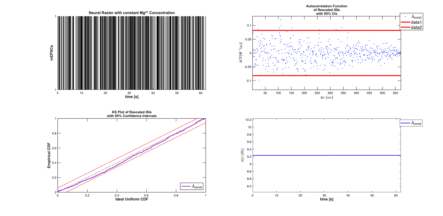
Under a constant Magnesium concentration, it is seen that the mEPSCs behave as a homogeneous poisson process (constant arrival rate).
    close all; clear all;
    [dataDir,mEPSCDir,explicitStimulusDir,psthDir,placeCellDataDir] = ...
        getPaperDataDirs();
    nSTATRootDir = fileparts(dataDir);
    if exist(nSTATRootDir,'dir') == 7 && ~strcmp(pwd,nSTATRootDir)
        cd(nSTATRootDir);
    end
    epsc2 = importdata(fullfile(mEPSCDir,'epsc2.txt'));
    sampleRate = 1000;
    spikeTimes = epsc2.data(:,2)*1/sampleRate; %in seconds
    nstConst = nspikeTrain(spikeTimes);
    time = 0:(1/sampleRate):nstConst.maxTime;


    % Define Covariates for the analysis
    baseline = Covariate(time,ones(length(time),1),'Baseline','time','s',...
        '',{'\mu'});
    covarColl = CovColl({baseline});

    % Create the trial structure
    spikeColl = nstColl(nstConst);
    trial     = Trial(spikeColl,covarColl);


    % Define how we want to analyze the data
    clear tc tcc;
    tc{1} = TrialConfig({{'Baseline','\mu'}},sampleRate,[]);
    tc{1}.setName('Constant Baseline');
    tcc = ConfigColl(tc);

    % Perform Analysis (Commented to since data already saved)
    results =Analysis.RunAnalysisForAllNeurons(trial,tcc,0);
%     h=results.plotResults;
    close all;
    scrsz = get(0,'ScreenSize');
    results.lambda.setDataLabels({'\lambda_{const}'});
    h=figure('OuterPosition',[scrsz(3)*.01 scrsz(4)*.04 ...
        scrsz(3)*.98 scrsz(4)*.95]);

    subplot(2,2,1); spikeColl.plot;
        title({'Neural Raster with constant Mg^{2+} Concentration'},...
            'FontWeight','bold',...
            'Fontsize',12,...
            'FontName','Arial');
         hx=xlabel('time [s]','Interpreter','none');
         hy=ylabel('mEPSCs','Interpreter','none');
         set(gca,'yTick',[0 1]);
         set([hx, hy],'FontName', 'Arial','FontSize',12,'FontWeight','bold');
    subplot(2,2,3); results.KSPlot;
    subplot(2,2,2); results.plotInvGausTrans;
    subplot(2,2,4); results.lambda.plot([],{{' ''b'' ,''Linewidth'',2'}});
    hx=xlabel('time [s]','Interpreter','none');
    hy=get(gca,'YLabel');
    set([hx hy],'FontName', 'Arial','FontSize',12,'FontWeight','bold');
    h_legend = legend('\lambda_{const}','Location','NorthEast');
    pos = get(h_legend,'position');
    set(h_legend, 'position',[pos(1)+.05 pos(2) pos(3:4)]);
    set(h_legend,'FontSize',14)
Analyzing Configuration #1: Neuron #1
Varying Magnesium Concentration - Piecewise Constant rate poisson
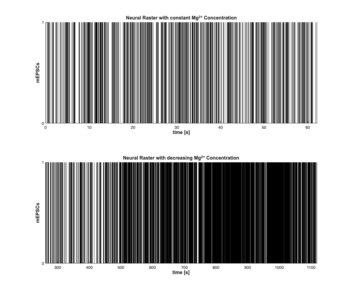
When the magnesium concentration of the bath decreased (i.e. magnesium is removed), the rate of mEPSCs begin to increase in frequency. This can be modeled in a many different ways (using the change in Magnesium directly as a model covariate, etc.) Here we approximate the rate as being constant during certain portions of the experiment. These segments can in principle be estimated (using heirarchical Bayesian methods), but here we select them via visual inspection. We compare three models: a constant rate model (from above), a piecewise constant rate model, and a piecewise constant rate model with history.
    close all;
 % load the data;
    washout1 = importdata(fullfile(mEPSCDir,'washout1.txt'));
    washout2 = importdata(fullfile(mEPSCDir,'washout2.txt'));

    sampleRate  = 1000;
    % Magnesium removed at t=0
    spikeTimes1 = 260+washout1.data(:,2)*1/sampleRate; %in seconds
    spikeTimes2 = sort(washout2.data(:,2))*1/sampleRate + 745;%in seconds
    nst = nspikeTrain([spikeTimes1; spikeTimes2]);
    time = 260:(1/sampleRate):nst.maxTime;
Data Visualization
Visual inspection of the spike train is used to pick three regions where the firing rate appears to be different. Here we do not estimate where these transitions happen but pick times in an ad-hoc manner.
    scrsz = get(0,'ScreenSize');
    h=figure('OuterPosition',[scrsz(3)*.01 scrsz(4)*.04 scrsz(3)*.6 ...
        scrsz(4)*.9]);

    subplot(2,1,1);
    nstConst.plot; set(gca,'yTick',[0 1]); hy=ylabel('mEPSCs');
     title({'Neural Raster with constant Mg^{2+} Concentration'},...
         'FontWeight','bold',...
            'Fontsize',12,...
            'FontName','Arial');
    hx=get(gca,'XLabel');
    set([hx,hy],'FontName', 'Arial','FontSize',12,'FontWeight','bold');

    subplot(2,1,2);
    nst.plot; set(gca,'yTick',[0 1]); hy=ylabel('mEPSCs');
    title({'Neural Raster with decreasing Mg^{2+} Concentration'},...
        'FontWeight','bold',...
            'Fontsize',12,...
            'FontName','Arial');
    hx=get(gca,'XLabel');
    set([hx,hy],'FontName', 'Arial','FontSize',12,'FontWeight','bold');
Define Covariates for the analysis
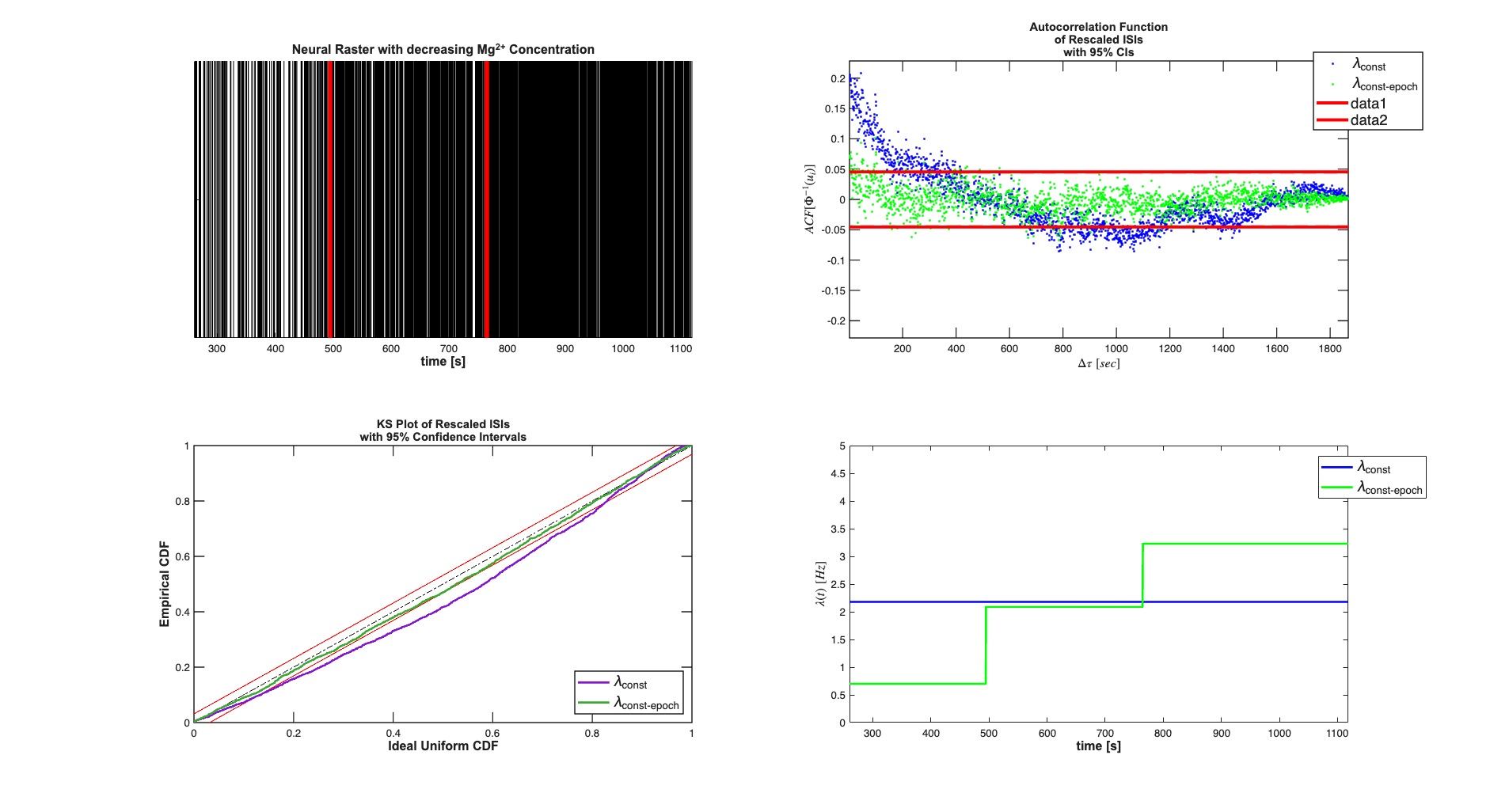
          timeInd1 =find(time<495,1,'last'); %0-495sec first constant rate
        timeInd2 =find(time<765,1,'last'); %495-765 second constant rate epoch
                                       %765 onwards third constant rate
                                       %epoch
    constantRate = ones(length(time),1);
    rate1 = zeros(length(time),1); rate1(1:timeInd1)=1;
    rate2 = zeros(length(time),1); rate2((timeInd1+1):timeInd2)=1;
    rate3 = zeros(length(time),1); rate3((timeInd2+1):end)=1;
    baseline = Covariate(time,[constantRate,rate1, rate2, rate3],...
        'Baseline','time','s','',{'\mu','\mu_{1}','\mu_{2}','\mu_{3}'});
    covarColl = CovColl({baseline});

    % Create the trial structure
    spikeColl = nstColl(nst);
    trial     = Trial(spikeColl,covarColl);

    %30ms history in logarithmic spacing (chosen after using
    %Analysis.computeHistLagForAll for various window lengths)
    maxWindow=.3; numWindows=20;
    delta=1/sampleRate;
    windowTimes =unique(round([0 logspace(log10(delta),...
    log10(maxWindow),numWindows)]*sampleRate)./sampleRate);
    windowTimes = windowTimes(1:11);
Define how we want to analyze the data
    clear tc tcc;
    tc{1} = TrialConfig({{'Baseline','\mu'}},sampleRate,[]);
    tc{1}.setName('Constant Baseline');
    tc{2} = TrialConfig({{'Baseline','\mu_{1}','\mu_{2}','\mu_{3}'}},...
        sampleRate,[]); tc{2}.setName('Diff Baseline');
    tcc = ConfigColl(tc);
Perform Analysis
We see that the piece-wise constant rate model (without history) outperforms the constant baseline model in terms of AIC, BIC, and KS-statistic.
    results =Analysis.RunAnalysisForAllNeurons(trial,tcc,0);
%     h=results.plotResults;
%     Summary = FitResSummary(results);
%     h=Summary.plotSummary;
Analyzing Configuration #1: Neuron #1
Analyzing Configuration #2: Neuron #1
close all;
    scrsz = get(0,'ScreenSize');
    results.lambda.setDataLabels({'\lambda_{const}',...
        '\lambda_{const-epoch}'});
    h=figure('OuterPosition',[scrsz(3)*.01 scrsz(4)*.04 ...
        scrsz(3)*.98 scrsz(4)*.95]);

    subplot(2,2,1); spikeColl.plot;
        title({'Neural Raster with decreasing Mg^{2+} Concentration'},...
            'FontWeight','bold',...
            'Fontsize',12,...
            'FontName','Arial');
        hx=xlabel('time [s]','Interpreter','none');
        set(gca,'YTickLabel',[]);
        set([hx],'FontName', 'Arial','FontSize',12,'FontWeight','bold');
        timeInd1 =find(time<495,1,'last'); %0-495sec first constant rate
        timeInd2 =find(time<765,1,'last'); %495-765 second constant rate epoch
                                       %765 onwards third constant rate
                                       %epoch
        plot([495;495],[0,1],'r','Linewidth',4); hold on;
        plot([765;765],[0,1],'r','Linewidth',4);

    subplot(2,2,3); results.KSPlot;
    subplot(2,2,2); results.plotInvGausTrans;
    subplot(2,2,4);
    results.lambda.getSubSignal(1).plot([],{{' ''b'' ,''Linewidth'',2'}});
    results.lambda.getSubSignal(2).plot([],{{' ''g'' ,''Linewidth'',2'}});
                    v=axis; axis([v(1) v(2) 0 5]);
    hx=xlabel('time [s]','Interpreter','none');
    hy=get(gca,'YLabel');
    set([hx hy],'FontName', 'Arial','FontSize',12,'FontWeight','bold');
    h_legend = legend('\lambda_{const}','\lambda_{const-epoch}',...
        'Location','NorthEast');
    pos = get(h_legend,'position');
    set(h_legend, 'position',[pos(1)+.05 pos(2)-.01 pos(3:4)]);
    set(h_legend,'FontSize',14)
Experiment 2
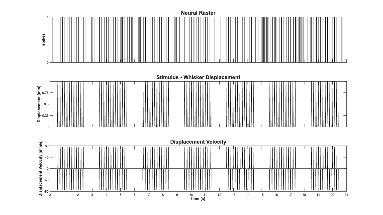
EXPLICIT STIMULUS EXAMPLE - WHISKER STIMULATION/THALAMIC NEURON In the worksheet with analyze the stimulus effect and history effect on the firing of a thalamic neuron under a known stimulus consisting of whisker stimulation. Data from Demba Ba (demba@mit.edu)
Load the data
clear all;
close all;
[dataDir,mEPSCDir,explicitStimulusDir,psthDir,placeCellDataDir] = ...
    getPaperDataDirs();
nSTATRootDir = fileparts(dataDir);
if exist(nSTATRootDir,'dir') == 7 && ~strcmp(pwd,nSTATRootDir)
    cd(nSTATRootDir);
end

Direction=3; Neuron=1; Stim=2;
datapath = fullfile(explicitStimulusDir,['Dir' num2str(Direction)], ...
    ['Neuron' num2str(Neuron)],['Stim' num2str(Stim)]);
data = load(fullfile(datapath,'trngdataBis.mat'));

time=0:.001:(length(data.t)-1)*.001;
stimData = data.t;
spikeTimes = time(data.y==1);

stim = Covariate(time,stimData./10,'Stimulus','time','s','mm',{'stim'});
baseline = Covariate(time,ones(length(time),1),'Baseline','time','s','',...
    {'constant'});

nst = nspikeTrain(spikeTimes);
nspikeColl = nstColl(nst);
cc = CovColl({stim,baseline});
trial = Trial(nspikeColl,cc);
% trial.plot;

scrsz = get(0,'ScreenSize');
h=figure('Position',[scrsz(3)*.1 scrsz(4)*.1 scrsz(3)*.8 scrsz(4)*.8]);
subplot(3,1,1);
nst2 = nspikeTrain(spikeTimes);
nst2.setMaxTime(21);nst2.plot;
set(gca,'ytick',[0 1]);
xlabel('');
hy=ylabel('spikes');
set(hy,'FontName', 'Arial','FontSize',12,'FontWeight','bold');
title({'Neural Raster'},'FontWeight','bold','FontSize',16,'FontName','Arial');
set(gca, ...
  'XTick'       , 0:1:max(time), ...
  'XTickLabel'  , [],...
  'LineWidth'   , 1         );
subplot(3,1,2);
stim.getSigInTimeWindow(0,21).plot([],{{' ''k'' '}}); legend off;
set(gca,'ytick',[0 0.5 1]);
hy=ylabel('Displacement [mm]','Interpreter','none'); xlabel('');
set(hy,'FontName', 'Arial','FontSize',12,'FontWeight','bold');
title({'Stimulus - Whisker Displacement'},'FontWeight','bold',...
    'FontSize',16,'FontName','Arial');

set(gca, ...
  'XTick'       , 0:1:max(time), ...
  'XTickLabel'  , [],...
  'YTick'       , 0:.25:1, ...
  'LineWidth'   , 1         );

subplot(3,1,3);
stim.derivative.getSigInTimeWindow(0,21).plot([],{{' ''k'' '}}); legend off;
set(gca,'ytick',[-80 0 80]);
axis([0 21 -80 80]);
hy=ylabel('Displacement Velocity [mm/s]','Interpreter','none');
hx= xlabel('time [s]','Interpreter','none');
set([hx hy],'FontName', 'Arial','FontSize',12,'FontWeight','bold');
title({'Displacement Velocity'},'FontWeight','bold',...
    'FontSize',16,'FontName','Arial');

set(gca, ...
  'XTick'       , 0:1:max(time), ...
  'YTick'       , -80:40:80, ...
  'LineWidth'   , 1         );
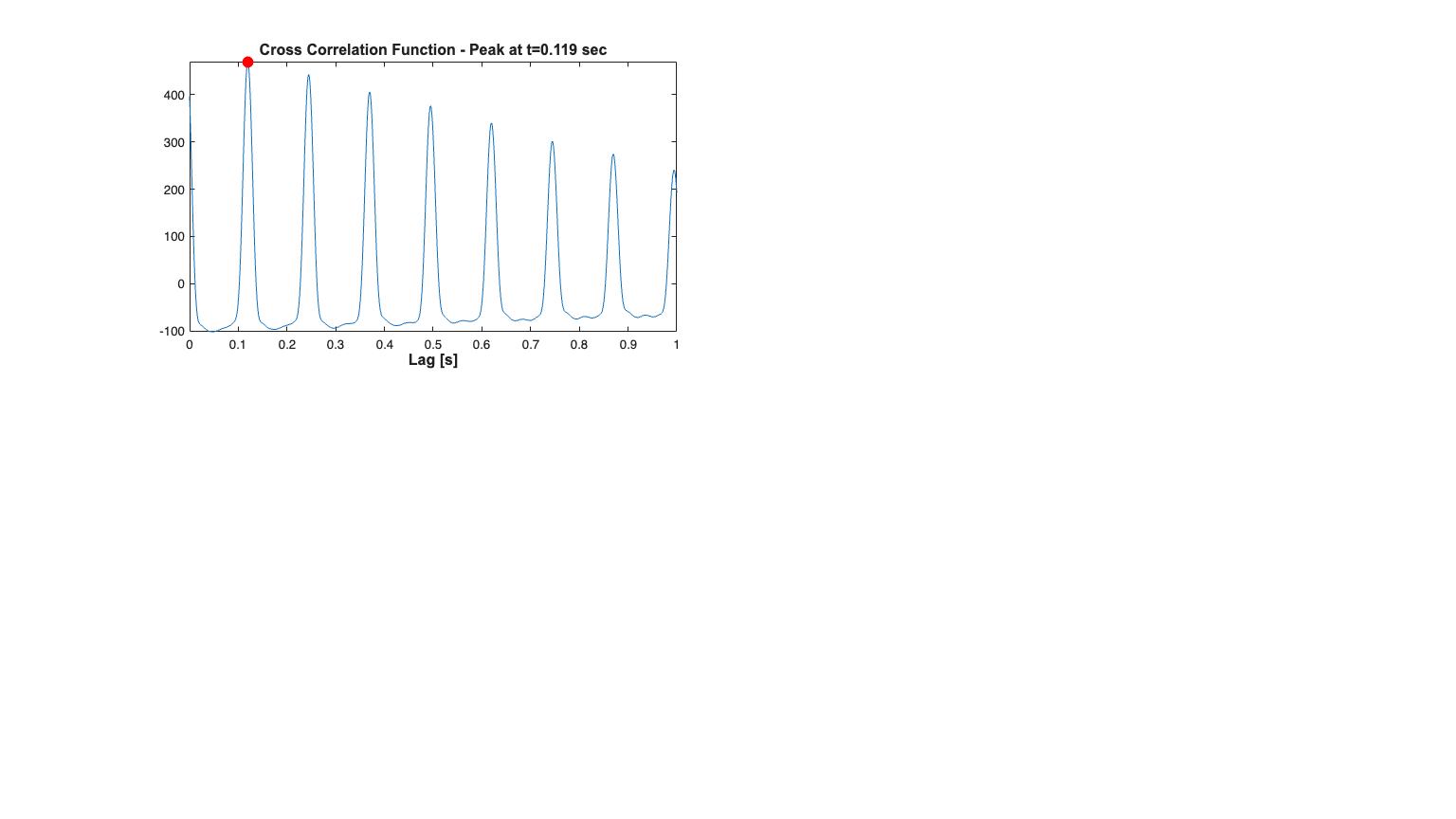
Fit a constant baseline and Find Stimulus Lag We fit a constant rate (Poisson) model to the data and use the look at the cross-covariance function of between the stimulus and the fit residual to determine the appropriate lag for the stimulus.
clear c; close all;
selfHist = [] ; NeighborHist = []; sampleRate = 1000;
c{1} = TrialConfig({{'Baseline','constant'}},sampleRate,selfHist,NeighborHist);
c{1}.setName('Baseline');
cfgColl= ConfigColl(c);
results = Analysis.RunAnalysisForAllNeurons(trial,cfgColl,0);

% Find Stimulus Lag (look for peaks in the cross-covariance function less
% than 1 second
scrsz = get(0,'ScreenSize');
h=figure('Position',[scrsz(3)*.1 scrsz(4)*.1 scrsz(3)*.8 scrsz(4)*.8]);

subplot(7,2,[1 3 5])
results.Residual.xcov(stim).windowedSignal([0,1]).plot;

ylabel('');
[m,ind,ShiftTime] = max(results.Residual.xcov(stim).windowedSignal([0,1]));
title(['Cross Correlation Function - Peak at t=' num2str(ShiftTime) ' sec'],'FontWeight','bold',...
            'FontSize',12,...
            'FontName','Arial');
hold on;
h=plot(ShiftTime,m,'ro','Linewidth',3);
set(h, 'MarkerFaceColor',[1 0 0], 'MarkerEdgeColor',[1 0 0]);
hx=xlabel('Lag [s]','Interpreter','none');
set(hx,'FontName', 'Arial','FontSize',12,'FontWeight','bold');


%Allow for shifts of less than 1 second
stim = Covariate(time,stimData,'Stimulus','time','s','V',{'stim'});
stim = stim.shift(ShiftTime);
baseline = Covariate(time,ones(length(time),1),'Baseline','time','s','',...
    {'\mu'});

nst = nspikeTrain(spikeTimes);
nspikeColl = nstColl(nst);
cc = CovColl({stim,baseline});
trial2 = Trial(nspikeColl,cc);
Analyzing Configuration #1: Neuron #1
Compare constant rate model with model including stimulus effect
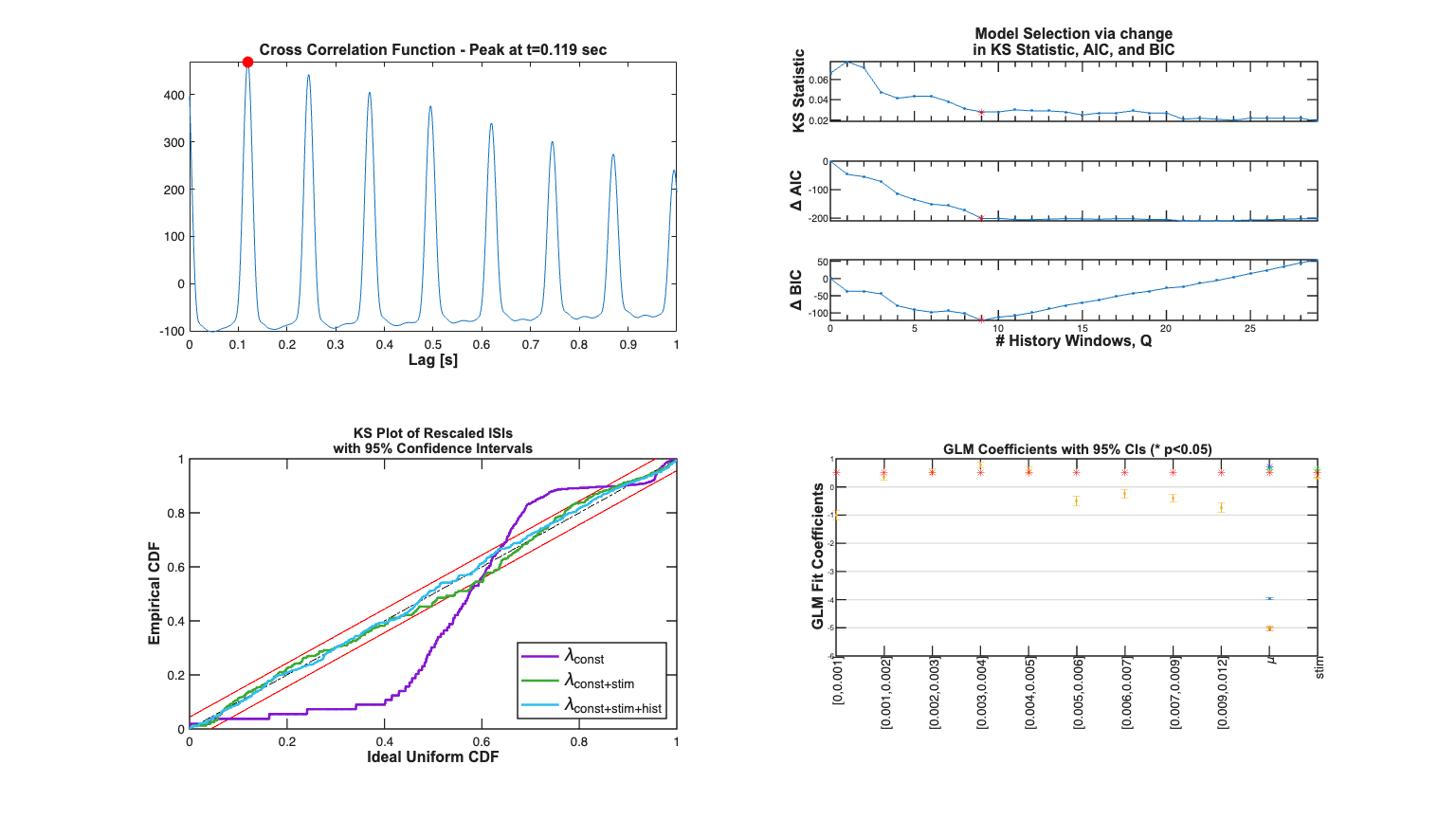
Addition of the stimulus improves the fits in terms of the KS plot and the making the rescaled ISIs less correlated. The Point Process Residula also looks more "white"
clear c;
selfHist = [] ; NeighborHist = []; sampleRate = 1000;
c{1} = TrialConfig({{'Baseline','\mu'}},sampleRate,selfHist,...
    NeighborHist);
c{1}.setName('Baseline');
c{2} = TrialConfig({{'Baseline','\mu'},{'Stimulus','stim'}},...
    sampleRate,selfHist,NeighborHist);
c{2}.setName('Baseline+Stimulus');
cfgColl= ConfigColl(c);
results = Analysis.RunAnalysisForAllNeurons(trial2,cfgColl,0);
% results.plotResults;
Analyzing Configuration #1: Neuron #1
Analyzing Configuration #2: Neuron #1
History Effect
Determine the best history effect model using AIC, BIC, and KS statistic
sampleRate=1000;
delta=1/sampleRate*1;
maxWindow=1; numWindows=32;
windowTimes =unique(round([0 logspace(log10(delta),...
    log10(maxWindow),numWindows)]*sampleRate)./sampleRate);
results =Analysis.computeHistLagForAll(trial2,windowTimes,...
    {{'Baseline','\mu'},{'Stimulus','stim'}},'BNLRCG',0,sampleRate,0);

KSind = find(results{1}.KSStats.ks_stat == min(results{1}.KSStats.ks_stat));
AICind = find((results{1}.AIC(2:end)-results{1}.AIC(1))== ...
               min(results{1}.AIC(2:end)-results{1}.AIC(1))) +1;
BICind = find((results{1}.BIC(2:end)-results{1}.BIC(1))== ...
               min(results{1}.BIC(2:end)-results{1}.BIC(1))) +1;
if(AICind==1)
    AICind=inf;
end
if(BICind==1)
    BICind=inf; %sometime BIC is non-decreasing and the index would be 1
end
windowIndex = min([AICind,BICind]) %use the minimum order model
Summary = FitResSummary(results);
% Summary.plotSummary;


clear c;
if(windowIndex>1)
    selfHist = windowTimes(1:windowIndex+1);
else
    selfHist = [];
end
NeighborHist = []; sampleRate = 1000;
%
% figure;
subplot(7,2,2);
x=0:length(windowTimes)-1;
plot(x,results{1}.KSStats.ks_stat,'.-'); axis tight; hold on;
plot(x(windowIndex),results{1}.KSStats.ks_stat(windowIndex),'r*');

 set(gca,'XTick', 0:5:results{1}.numResults-1,'XTickLabel',[],...
     'TickLength', [.02 .02] , ...
  'XMinorTick', 'on','LineWidth'   , 1);

hy=ylabel('KS Statistic');
set(hy,'FontName', 'Arial','FontSize',12,'FontWeight','bold');
dAIC = results{1}.AIC-results{1}.AIC(1);
 title({'Model Selection via change'; 'in KS Statistic, AIC, and BIC'},...
     'FontWeight','bold',...
            'FontSize',12,...
            'FontName','Arial');

subplot(7,2,4); plot(x,dAIC,'.-');
set(gca,'XTick', 0:5:results{1}.numResults-1,'XTickLabel',[],...
     'TickLength', [.02 .02] , ...
  'XMinorTick', 'on','LineWidth'   , 1);
hy=ylabel('\Delta AIC');axis tight; hold on;
set(hy,'FontName', 'Arial','FontSize',12,'FontWeight','bold');
plot(x(windowIndex),dAIC(windowIndex),'r*');
dBIC = results{1}.BIC-results{1}.BIC(1);

subplot(7,2,6); plot(x,dBIC,'.-');
hy=ylabel('\Delta BIC'); axis tight; hold on;

plot(x(windowIndex),dBIC(windowIndex),'r*');
hx=xlabel('# History Windows, Q');
set([hx, hy],'FontName', 'Arial','FontSize',12,'FontWeight','bold');
set(gca, ...
  'TickLength'  , [.02 .02] , ...
  'XMinorTick'  , 'on'      , ...
  'XTick'       , 0:5:results{1}.numResults-1, ...
  'LineWidth'   , 1         );


% Compare Baseline, Baseline+Stimulus Model, Baseline+History+Stimulus
% Addition of the history effect yields a model that falls within the 95%
% CI of the KS plot.

c{1} = TrialConfig({{'Baseline','\mu'}},sampleRate,[],NeighborHist);
c{1}.setName('Baseline');
c{2} = TrialConfig({{'Baseline','\mu'},{'Stimulus','stim'}},...
                    sampleRate,[],[]);
c{2}.setName('Baseline+Stimulus');
c{3} = TrialConfig({{'Baseline','\mu'},{'Stimulus','stim'}},...
                    sampleRate,windowTimes(1:windowIndex),[]);
c{3}.setName('Baseline+Stimulus+Hist');
cfgColl= ConfigColl(c);
results = Analysis.RunAnalysisForAllNeurons(trial2,cfgColl,0);
%results.plotResults;
%
results.lambda.setDataLabels({'\lambda_{const}','\lambda_{const+stim}',...
    '\lambda_{const+stim+hist}'});
subplot(7,2,[9 11 13]); results.KSPlot;
subplot(7,2,[10 12 14]); results.plotCoeffs; legend off;
Analyzing Configuration #1: Neuron #1
Analyzing Configuration #2: Neuron #1
Analyzing Configuration #3: Neuron #1
Analyzing Configuration #4: Neuron #1
Analyzing Configuration #5: Neuron #1
Analyzing Configuration #6: Neuron #1
Analyzing Configuration #7: Neuron #1
Analyzing Configuration #8: Neuron #1
Analyzing Configuration #9: Neuron #1
Analyzing Configuration #10: Neuron #1
Analyzing Configuration #11: Neuron #1
Analyzing Configuration #12: Neuron #1
Analyzing Configuration #13: Neuron #1
Analyzing Configuration #14: Neuron #1
Analyzing Configuration #15: Neuron #1
Analyzing Configuration #16: Neuron #1
Analyzing Configuration #17: Neuron #1
Analyzing Configuration #18: Neuron #1
Analyzing Configuration #19: Neuron #1
Analyzing Configuration #20: Neuron #1
Analyzing Configuration #21: Neuron #1
Analyzing Configuration #22: Neuron #1
Analyzing Configuration #23: Neuron #1
Analyzing Configuration #24: Neuron #1
Analyzing Configuration #25: Neuron #1
Analyzing Configuration #26: Neuron #1
Analyzing Configuration #27: Neuron #1
Analyzing Configuration #28: Neuron #1
Analyzing Configuration #29: Neuron #1
Analyzing Configuration #30: Neuron #1

windowIndex =

    10

Analyzing Configuration #1: Neuron #1
Analyzing Configuration #2: Neuron #1
Analyzing Configuration #3: Neuron #1
Example 3 - PSTH Data
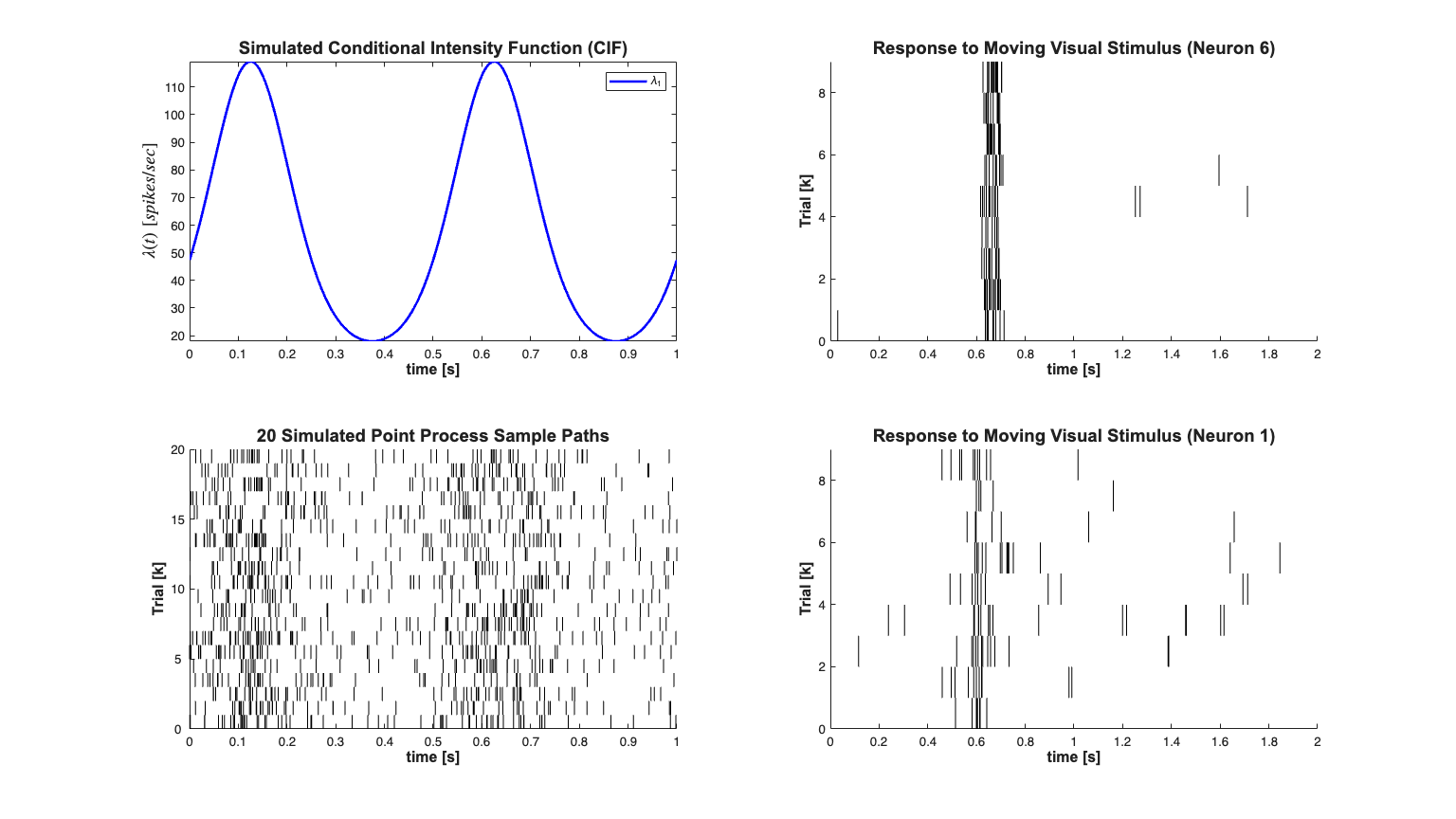
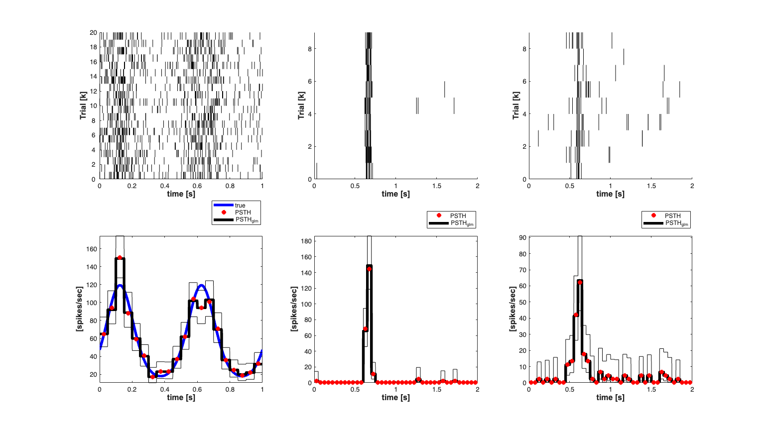
% Generate a known Conditional Intensity Function
% We generated a known conditional intensity function (rate function) and
% generate distinct realizations of point processes consistent with this
% rate function. We use the method of thinning to simulate a point process.
clear all;
[dataDir,mEPSCDir,explicitStimulusDir,psthDir,placeCellDataDir] = ...
    getPaperDataDirs();
close all;
delta = 0.001;
Tmax = 1;
time = 0:delta:Tmax;
f=2;
mu = -3;

tempData = 1*sin(2*pi*f*time)+mu; %lambda >=0
lambdaData = exp(tempData)./(1+exp(tempData))*(1/delta);
lambda = Covariate(time,lambdaData, '\lambda(t)','time','s',...
    'spikes/sec',{'\lambda_{1}'},{{' ''b'', ''LineWidth'' ,2'}});
numRealizations = 20;
spikeCollSim = CIF.simulateCIFByThinningFromLambda(lambda,numRealizations);


scrsz = get(0,'ScreenSize');
h=figure('Position',[scrsz(3)*.1 scrsz(4)*.1 scrsz(3)*.8 scrsz(4)*.8]);

subplot(2,2,3);spikeCollSim.plot;
set(gca,'YTick',0:5:numRealizations,'YTickLabel',0:5:numRealizations);
title({[num2str(numRealizations) ' Simulated Point Process Sample Paths']},...
    'FontWeight','bold','Fontsize',14,'FontName','Arial');
xlabel('time [s]','Interpreter','none','FontName', 'Arial',...
    'Fontsize',12,'FontWeight','bold');
ylabel('Trial [k]','Interpreter','none','FontName', 'Arial',...
    'Fontsize',12,'FontWeight','bold');

subplot(2,2,1);lambda.plot;
title({'Simulated Conditional Intensity Function (CIF)'},...
    'FontWeight','bold','FontSize',14,'FontName','Arial');
xlabel('time [s]','Interpreter','none','FontName', 'Arial',...
    'Fontsize',12,'FontWeight','bold');
hy=get(gca,'YLabel');
set(hy,'FontName', 'Arial','FontSize',14,'FontWeight','bold');

x = load(fullfile(psthDir,'Results.mat'));
numTrials = x.Results.Data.Spike_times_STC.balanced_SUA.Nr_trials;
cellNum=6; clear nst;
for i=1:numTrials
    spikeTimes{i}=x.Results.Data.Spike_times_STC.balanced_SUA.spike_times{1,i,cellNum};
    nst{i} = nspikeTrain(spikeTimes{i});
    nst{i}.setName(num2str(cellNum));
end

spikeCollReal1=nstColl(nst);
spikeCollReal1.setMinTime(0); spikeCollReal1.setMaxTime(2);
subplot(2,2,2);spikeCollReal1.plot;  set(gca,'YTick',0:2:numTrials,...
    'YTickLabel',0:2:numTrials);
%set(gca,'xtick',[0:.5:2],'xtickLabel',{'0','0.5','1','1.5','2'});
xlabel('time [s]','Interpreter','none','FontName', 'Arial',...
    'Fontsize',12,'FontWeight','bold');
ylabel('Trial [k]','Interpreter','none','FontName', 'Arial',...
    'Fontsize',12,'FontWeight','bold');
title('Response to Moving Visual Stimulus (Neuron 6)',...
    'FontWeight','bold','Fontsize',14,'FontName','Arial');

cellNum=1; clear nst;
for i=1:numTrials
    spikeTimes{i}=x.Results.Data.Spike_times_STC.balanced_SUA.spike_times{1,i,cellNum};
    nst{i} = nspikeTrain(spikeTimes{i});
    nst{i}.setName(num2str(cellNum));
end

spikeCollReal2=nstColl(nst);
spikeCollReal2.setMinTime(0); spikeCollReal2.setMaxTime(2);
subplot(2,2,4);spikeCollReal2.plot;
set(gca,'YTick',0:2:numTrials,'YTickLabel',0:2:numTrials);
%set(gca,'xtick',[0:.5:2],'xtickLabel',{'0','0.5','1','1.5','2'});
xlabel('time [s]','Interpreter','none','FontName', 'Arial',...
    'Fontsize',12,'FontWeight','bold');
ylabel('Trial [k]','Interpreter','none','FontName', 'Arial',...
    'Fontsize',12,'FontWeight','bold');
title('Response to Moving Visual Stimulus (Neuron 1)','FontWeight',...
    'bold','Fontsize',14,'FontName','Arial');
Estimate the PSTH with 50ms windows
close all;

scrsz = get(0,'ScreenSize');
h=figure('Position',[scrsz(3)*.1 scrsz(4)*.1 scrsz(3)*.8 scrsz(4)*.8]);

binsize = .05; %50ms window
psth    = spikeCollSim.psth(binsize);
psthGLM = spikeCollSim.psthGLM(binsize);
true = lambda; %rate*delta = expected number of arrivals per bin
subplot(2,3,4);

h1=true.plot([],{{' ''b'',''Linewidth'',4'}});
h3=psthGLM.plot([],{{' ''k'',''Linewidth'',4'}});
h2=psth.plot([],{{' ''rx'',''Linewidth'',4'}});

xlabel('time [s]','Interpreter','none','FontName', 'Arial',...
    'Fontsize',12,'FontWeight','bold');
ylabel('[spikes/sec]','Interpreter','none','FontName', 'Arial',...
    'Fontsize',12,'FontWeight','bold');

legend off;
h_legend=legend([h1(1) h2(1)  h3(1)],'true','PSTH','PSTH_{glm}');
pos = get(h_legend,'position');
set(h_legend, 'position',[pos(1)+.005 pos(2)+.095 pos(3:4)]);


%
subplot(2,3,1);spikeCollSim.plot;
set(gca,'YTick',0:2:spikeCollSim.numSpikeTrains,'YTickLabel',0:2:spikeCollSim.numSpikeTrains);
xlabel('time [s]','Interpreter','none','FontName', 'Arial','Fontsize',...
    12,'FontWeight','bold');
ylabel('Trial [k]','Interpreter','none','FontName', 'Arial',...
    'Fontsize',12,'FontWeight','bold');

subplot(2,3,5);
binsize = .05; %50ms window
psthReal1    = spikeCollReal1.psth(binsize);
psthGLMReal1 = spikeCollReal1.psthGLM(binsize);%,[],[],[],[],[],1000);

h3=psthGLMReal1.plot([],{{' ''k'',''Linewidth'',4'}});
h2=psthReal1.plot([],{{' ''rx'',''Linewidth'',4'}});
xlabel('time [s]','Interpreter','none','FontName', 'Arial','Fontsize',...
    12,'FontWeight','bold');
ylabel('[spikes/sec]','Interpreter','none','FontName', 'Arial','Fontsize',...
    12,'FontWeight','bold');

h_legend=legend([h2(1)  h3(1)],'PSTH','PSTH_{glm}');
pos = get(h_legend,'position');
set(h_legend, 'position',[pos(1)+.005 pos(2)+.07 pos(3:4)]);
subplot(2,3,2); spikeCollReal1.plot;
set(gca,'YTick',0:2:spikeCollReal2.numSpikeTrains,'YTickLabel',0:2:spikeCollReal2.numSpikeTrains);
xlabel('time [s]','Interpreter','none','FontName', 'Arial','Fontsize',...
    12,'FontWeight','bold');
ylabel('Trial [k]','Interpreter','none','FontName', 'Arial',...
    'Fontsize',12,'FontWeight','bold');
subplot(2,3,6);
psthReal2    = spikeCollReal2.psth(binsize);
psthGLMReal2 = spikeCollReal2.psthGLM(binsize);%,[],[],[],[],[],1000);
h3=psthGLMReal2.plot([],{{' ''k'',''Linewidth'',4'}});
h2=psthReal2.plot([],{{' ''rx'',''Linewidth'',4'}});
xlabel('time [s]','Interpreter','none','FontName', 'Arial','Fontsize',...
    12,'FontWeight','bold');
ylabel('[spikes/sec]','Interpreter','none','FontName', 'Arial','Fontsize',...
    12,'FontWeight','bold');


h_legend=legend([h2(1)  h3(1)],'PSTH','PSTH_{glm}');
pos = get(h_legend,'position');
set(h_legend, 'position',[pos(1)+.005 pos(2)+.07 pos(3:4)]);
subplot(2,3,3); spikeCollReal2.plot;
set(gca,'YTick',0:2:spikeCollReal2.numSpikeTrains,'YTickLabel',0:2:spikeCollReal2.numSpikeTrains);
xlabel('time [s]','Interpreter','none','FontName', 'Arial','Fontsize',...
    12,'FontWeight','bold');
ylabel('Trial [k]','Interpreter','none','FontName', 'Arial',...
    'Fontsize',12,'FontWeight','bold');
Running in batch mode: neurons with same name are fit simultaneously
Analyzing Configuration #1: Neuron #1
Running in batch mode: neurons with same name are fit simultaneously
Analyzing Configuration #1: Neuron #6
Running in batch mode: neurons with same name are fit simultaneously
Analyzing Configuration #1: Neuron #1
Example 3b - SSGLM Example
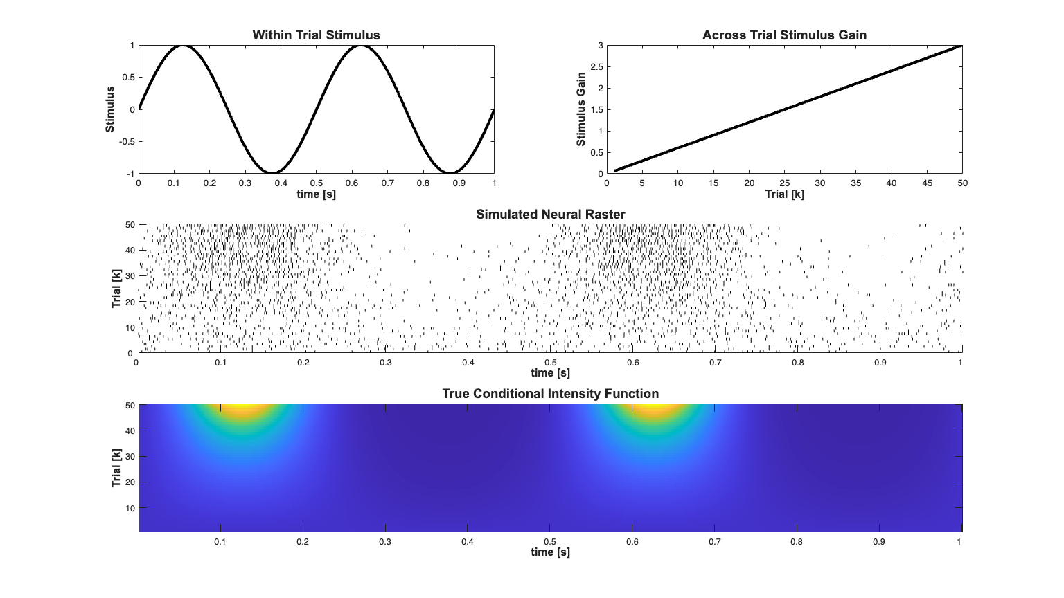
Example of estimating with-in and across trial dynamics Methods from: G. Czanner, U. T. Eden, S. Wirth, M. Yanike, W. A. Suzuki, and E. N. Brown, "Analysis of between-trial and within-trial neural spiking dynamics.," Journal of neurophysiology, vol. 99, no. 5, pp. 2672?2693, May. 2008.
close all;
clear all;
[dataDir,mEPSCDir,explicitStimulusDir,psthDir,placeCellDataDir] = ...
    getPaperDataDirs();
% set(0,'DefaultFigureRenderer','ZBuffer')
delta = 0.001; Tmax = 1;
time = 0:delta:Tmax;
Ts=.001;
numRealizations = 50; %Each realization corresponds to a distinct trial

for i=1:numRealizations
    % The within trial dynamics are sinusoidal
    % For each trial the stimulus effect increases
    f=2; b1(i)=3*((i)/numRealizations);b0=-3;
    u = sin(2*pi*f*time);
    e = zeros(length(time),1);   %No Ensemble input

    stim=Covariate(time',u,'Stimulus','time','s','Voltage',{'sin'});
    ens =Covariate(time',e,'Ensemble','time','s','Spikes',{'n1'});

    mu=b0;
    histCoeffs=[-4 -1 -.5];
    H=tf(histCoeffs,[1],Ts,'Variable','z^-1');

    S=tf([b1(i)],1,Ts,'Variable','z^-1');
    E=tf([0],1,Ts,'Variable','z^-1');
    simTypeSelect='binomial'; %Parameters are used to compute
                              %binomial conditional intensity function
                              %

    % Obtain a realization of the point process with the current
    % stimulus and history effect
    [sC, lambdaTemp]=CIF.simulateCIF(mu,H,S,E,stim,ens,1,simTypeSelect);

    if(i==1)
        lambda=lambdaTemp; %Store the conditional intensity function
    else
        lambda = lambda.merge(lambdaTemp); %Add it to the other realizations
    end

    nst{i} = sC.getNST(1);             %get the neural spikeTrain from the collection
    nst{i} = nst{i}.resample(1/delta); %make sure that it is sampled at the current samplerate
end

spikeColl = nstColl(nst); %Create a collection of the spike trains across trials
Summarize Simulated Data
close all;
scrsz = get(0,'ScreenSize');
h=figure('Position',[scrsz(3)*.1 scrsz(4)*.1 scrsz(3)*.8 scrsz(4)*.8]);

%Plot the raster
subplot(3,2,[3 4]); spikeColl.plot;
set(gca,'ytick',0:10:numRealizations,'ytickLabel',0:10:numRealizations);
set(gca,'xtick',0:.1:Tmax,'xtickLabel',0:.1:Tmax); xlabel('');
xlabel('time [s]','Interpreter','none','FontName', 'Arial','Fontsize',...
    12,'FontWeight','bold');
ylabel('Trial [k]','Interpreter','none','FontName', 'Arial','Fontsize',...
    12,'FontWeight','bold');
title('Simulated Neural Raster','Interpreter','none','FontName', 'Arial',...
    'Fontsize',14,'FontWeight','bold');

% Plot the actual stimulus effect (not including history)
% The CIF including the history effect is stored in the lambda Covariate
% above


stimData = exp(b0 + u'*b1);
if(strcmp(simTypeSelect,'binomial'))
    stimData = stimData./(1+stimData);
end

%Plot the trial dependence
subplot(3,2,1); plot(time,u,'k','LineWidth',3);
% xlabel('time [s]');ylabel('stimulus');
xlabel('time [s]','Interpreter','none','FontName', 'Arial','Fontsize',...
    12,'FontWeight','bold');
ylabel('Stimulus','Interpreter','none','FontName', 'Arial','Fontsize',...
    12,'FontWeight','bold');
title('Within Trial Stimulus','Interpreter','none','FontName', 'Arial',...
    'Fontsize',14,'FontWeight','bold');

subplot(3,2,2); plot(1:length(b1),b1,'k','LineWidth',3);
xlabel('Trial [k]','Interpreter','none','FontName', 'Arial','Fontsize',...
    12,'FontWeight','bold');
ylabel('Stimulus Gain','Interpreter','none','FontName', 'Arial','Fontsize',...
    12,'FontWeight','bold');
title('Across Trial Stimulus Gain','Interpreter','none','FontName',...
    'Arial','Fontsize',14,'FontWeight','bold');

subplot(3,2,[5 6]);
imagesc(stimData'./delta);  set(gca, 'YDir','normal');
set(gca,'xtick',0:100:Tmax/delta,'xtickLabel',0:.1:Tmax);
set(gca,'ytick',0:10:numRealizations,'ytickLabel',0:10:numRealizations);
xlabel('time [s]','Interpreter','none','FontName', 'Arial',...
    'Fontsize',12,'FontWeight','bold');
ylabel('Trial [k]','Interpreter','none','FontName', 'Arial',...
    'Fontsize',12,'FontWeight','bold');
title('True Conditional Intensity Function','Interpreter',...
    'none','FontName', 'Arial','Fontsize',14,'FontWeight','bold');


axis tight;
Estimation of the Stimulus Response
% Create the covariates that will be used for the GLM regression
stim = Covariate(time,sin(2*pi*f*time),'Stimulus','time','s','V',{'stim'});
baseline = Covariate(time,ones(length(time),1),'Baseline','time','s','',...
                    {'constant'});

% Specify the windows of the history coefficients to be estimated
windowTimes=[0:.001:.003];
% Number of bins to discrtize time into (used both for the PSTH and for
% thec
% SSGLM model.
numBasis = 25;

spikeColl.resample(1/delta); % Enforce sampleRate
spikeColl.setMaxTime(Tmax);  % Make all spikeTrains end at time Tmax


dN=spikeColl.dataToMatrix';  % Convert the spikeTrains into a matrix
                             % of 1's and 0's corresponding to the presence
                             % or absense of a spike in each time window.
dN(dN>1)=1;                  % One should sample finely enough so there is
                             % one spike per bin. Here we make sure that
                             % this is the case regardless of the
                             % sampleRate

% The width of each rectangular basis pulse is determined by Tmax and by the
% number of basis pulses to use.
basisWidth=(spikeColl.maxTime-spikeColl.minTime)/numBasis;

if(simTypeSelect==0)
    fitType='binomial';
else
    fitType='poisson';
end
if(strcmp(fitType,'binomial'))
    Algorithm = 'BNLRCG';   % BNLRCG - faster Truncated, L-2 Regularized,
                            % Binomial Logistic Regression with Conjugate
                            % Gradient Solver by Demba Ba (demba@mit.edu).
else
    Algorithm = 'GLM';      % Standard Matlab GLM (Can be used for binomial or
                            % or Poisson CIFs
end

% Use the values obtained from a PSTH to initialize the SSGLM filter
[psthSig, ~, psthResult] =spikeColl.psthGLM(basisWidth,windowTimes,fitType);
gamma0=psthResult.getHistCoeffs';%+.1*randn(size(histCoeffs));
gamma0(isnan(gamma0))=-5; % Depending on the amount of data the
                          % the psth may not identify all parameters
                          % Just make sure that the estimates are real
                          % numbers

x0=psthResult.getCoeffs;  %The initial estimate for the SSGLM model

% Estimate the variance within each time bin across trials
numVarEstIter=10;
Q0 = spikeColl.estimateVarianceAcrossTrials(numBasis,windowTimes,...
    numVarEstIter,fitType);
A=eye(numBasis,numBasis);
delta = 1/spikeColl.sampleRate;
Running in batch mode: neurons with same name are fit simultaneously
Analyzing Configuration #1: Neuron #1
Running in batch mode: neurons with same name are fit simultaneously
Analyzing Configuration #1: Neuron #1
Running in batch mode: neurons with same name are fit simultaneously
Analyzing Configuration #1: Neuron #1
Running in batch mode: neurons with same name are fit simultaneously
Analyzing Configuration #1: Neuron #1
Running in batch mode: neurons with same name are fit simultaneously
Analyzing Configuration #1: Neuron #1
Running in batch mode: neurons with same name are fit simultaneously
Analyzing Configuration #1: Neuron #1
Running in batch mode: neurons with same name are fit simultaneously
Analyzing Configuration #1: Neuron #1
Running in batch mode: neurons with same name are fit simultaneously
Analyzing Configuration #1: Neuron #1
Running in batch mode: neurons with same name are fit simultaneously
Analyzing Configuration #1: Neuron #1
Running in batch mode: neurons with same name are fit simultaneously
Analyzing Configuration #1: Neuron #1
Running in batch mode: neurons with same name are fit simultaneously
Analyzing Configuration #1: Neuron #1
A=eye(numBasis,numBasis);
delta = 1/spikeColl.sampleRate;
Run the SSGLM Filter
CompilingHelpFile=1;
    % Commented out to speed up help file creation ...
    if(~CompilingHelpFile)
        Q0d=diag(Q0);
        neuronName = psthResult.neuronNumber;
        [xK,WK, WkuFinal,Qhat,gammahat,fitResults,stimulus,stimCIs,logll,...
            QhatAll,gammahatAll,nIter]=nstat.decoding.SSGLM.PPSS_EMFB(A,Q0d,x0,...
            dN,fitType,delta,gamma0,windowTimes, numBasis,neuronName);

        fR = fitResults.toStructure;
        psthR = psthResult.toStructure;
    end
% save SSGLMExampleData psthR fR xK WK WkuFinal Qhat gammahat fitResults stimulus stimCIs logll QhatAll gammahatAll nIter;
%% Run the SSGLM Filter
CompilingHelpFile=1;
    % Commented out to speed up help file creation ...
    if(~CompilingHelpFile)
    end
installPath = which('nSTAT_Install');
if isempty(installPath)
    error('nSTATPaperExamples:MissingInstallPath', ...
        'Could not locate nSTAT_Install.m on MATLAB path.');
end
nstatRoot = fileparts(installPath);
if exist(nstatRoot,'dir') == 7 && ~strcmp(pwd,nstatRoot)
    cd(nstatRoot);
end
addpath(nstatRoot,'-begin');
load(fullfile(nstatRoot,'data','SSGLMExampleData.mat'));
fitResults = FitResult.fromStructure(fR);
psthResult = FitResult.fromStructure(psthR);
% save SSGLMExampleData psthR fR xK WK WkuFinal Qhat gammahat fitResults stimulus stimCIs logll QhatAll gammahatAll nIter;
%%
installPath = which('nSTAT_Install');
if isempty(installPath)
        'Could not locate nSTAT_Install.m on MATLAB path.');
end
nstatRoot = fileparts(installPath);
if exist(nstatRoot,'dir') == 7 && ~strcmp(pwd,nstatRoot)
end
addpath(nstatRoot,'-begin');
load(fullfile(nstatRoot,'data','SSGLMExampleData.mat'));
fitResults = FitResult.fromStructure(fR);
psthResult = FitResult.fromStructure(psthR);
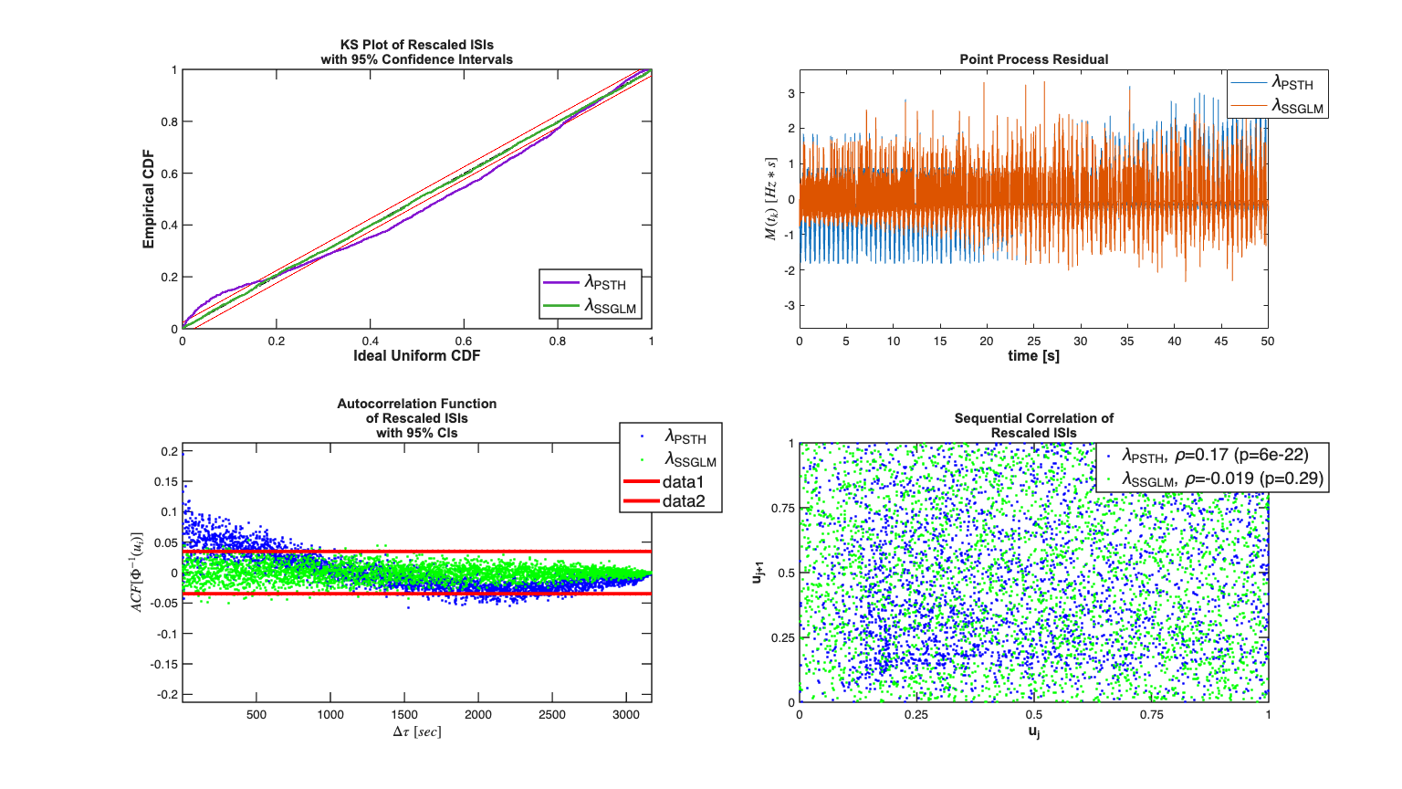
t=psthResult.mergeResults(fitResults);
%t.plotResults; %Compare the results with the PSTH Model
t.lambda.setDataLabels({'\lambda_{PSTH}','\lambda_{SSGLM}'});
scrsz = get(0,'ScreenSize');
h=figure('Position',[scrsz(3)*.1 scrsz(4)*.1 scrsz(3)*.8 scrsz(4)*.8]);
subplot(2,2,1); t.KSPlot;
subplot(2,2,2); t.plotResidual;
subplot(2,2,3); t.plotInvGausTrans;
subplot(2,2,4); t.plotSeqCorr;

S=FitResSummary(t);
dAIC=diff(S.AIC)
dBIC=diff(S.BIC)
dKS =diff(S.KSStats);
%%
t=psthResult.mergeResults(fitResults);
%t.plotResults; %Compare the results with the PSTH Model
t.lambda.setDataLabels({'\lambda_{PSTH}','\lambda_{SSGLM}'});
scrsz = get(0,'ScreenSize');
h=figure('Position',[scrsz(3)*.1 scrsz(4)*.1 scrsz(3)*.8 scrsz(4)*.8]);
subplot(2,2,1); t.KSPlot;
subplot(2,2,2); t.plotResidual;
subplot(2,2,3); t.plotInvGausTrans;
subplot(2,2,4); t.plotSeqCorr;

S=FitResSummary(t);
dAIC=diff(S.AIC)

dAIC =

  -1.7978e+04

dBIC=diff(S.BIC)

dBIC =

  -6.9523e+03

dKS =diff(S.KSStats);
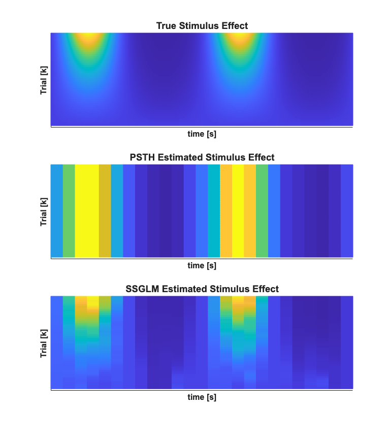
close all;
% Generate the actual stimulus effect
minTime=0; maxTime = Tmax;
stimData = stim.data*b1;
if(strcmp(fitType,'poisson'))
    actStimEffect=exp(stimData + b0)./delta;
elseif(strcmp(fitType,'binomial'))
    actStimEffect=exp(stimData + b0)./(1+exp(stimData + b0))./delta;
end
%

% Generate the basis function so that the estimated effect can be plotted
% at the same temporal resolution as the theoretical effect
 if(~isempty(numBasis))
    basisWidth = (maxTime-minTime)/numBasis;
    sampleRate=1/delta;
    unitPulseBasis=nstColl.generateUnitImpulseBasis(basisWidth,minTime,...
        maxTime,sampleRate);
    basisMat = unitPulseBasis.data;
 end

% Generate the estimated stimulus effect
if(strcmp(fitType,'poisson'))
    estStimEffect=exp(basisMat*xK)./delta;
elseif(strcmp(fitType,'binomial'))
    estStimEffect=exp(basisMat*xK)./(1+exp(basisMat*xK))./delta;
end


scrsz = get(0,'ScreenSize');
h=figure('OuterPosition',[scrsz(3)*.1 scrsz(4)*.1 scrsz(3)*.4 scrsz(4)*.8]);

% Plot the actual and estimated stimulus effect as a function of trial and
% time
subplot(3,1,[1 2 3]);
lighting gouraud
surf((1:length(b1))',stim.time,actStimEffect,'FaceAlpha',0.1,...
    'EdgeAlpha',0.1,'AlphaData',0.1);
hx=xlabel('Trial [k]'); hy=ylabel('time [s]');
hz=zlabel('Stimulus Effect [spikes/sec]'); hold all;
set([hx hy hz],'FontName', 'Arial','FontSize',12,'FontWeight','bold');

surf((1:length(b1))',stim.time,estStimEffect(:,1:length(b1)),...
    'FaceAlpha',0.5,'EdgeAlpha',0.1,'AlphaData',0.5); %xlabel('Trial [k]'); ylabel('time [s]'); zlabel('Stimulus Effect');
set(gca,'YDir','reverse');
set(gca,'ytick',0:.1:Tmax,'ytickLabel',0:.1:Tmax);

title('SSGLM Estimated vs. Actual Stimulus Effect','FontWeight','bold',...
            'Fontsize',14,...
            'FontName','Arial');

close all;
h=figure('OuterPosition',[scrsz(3)*.1 scrsz(4)*.1 scrsz(3)*.4 scrsz(4)*.8]);

% The actual stimulus effect
subplot(3,1,1);
lighting gouraud
mesh((1:length(b1))',stim.time,actStimEffect);
hx=xlabel('Trial [k]'); hy=ylabel('time [s]');
zlabel('Stimulus Effect [spikes/sec]'); hold all;
set([hx hy],'FontName', 'Arial','FontSize',12,'FontWeight','bold');
% title('True Stimulus Effect');
title('True Stimulus Effect','FontWeight','bold',...
            'Fontsize',14,...
            'FontName','Arial');
set(gca,'xtick',[],'xtickLabel',[]);
set(gca,'ytick',[],'ytickLabel',[]);
CLIM = [min(min(stimData./delta)) max(max(stimData./delta))];
view(gca,[90 -90]);


% The PSTH estimate
subplot(3,1,2);
lighting gouraud
mesh((1:length(b1))',stim.time,repmat(psthSig.data, [1 numRealizations]));
hx=xlabel('Trial [k]'); hy=ylabel('time [s]');
hz=zlabel('Stimulus Effect [spikes/sec]'); hold all;
set([hx hy hz],'FontName', 'Arial','FontSize',12,'FontWeight','bold');
% title('PSTH Estimated Stimulus Effect');
title('PSTH Estimated Stimulus Effect','FontWeight','bold',...
            'Fontsize',14,...
            'FontName','Arial');

set(gca,'xtick',[],'xtickLabel',[]);
set(gca,'ytick',[],'ytickLabel',[]);
CLIM = [min(min(stimData./delta)) max(max(stimData./delta))];
view(gca,[90 -90]);

% The SSGLM estimated stimulus effect
subplot(3,1,3);
lighting gouraud
mesh((1:length(b1))',stim.time,estStimEffect);
xlabel('Trial [k]'); ylabel('time [s]');
zlabel('Stimulus Effect [spikes/sec]'); hold all;
hx=get(gca,'XLabel');  hy=get(gca,'YLabel'); hz=get(gca,'ZLabel');
set([hx hy hz],'FontName', 'Arial','FontSize',12,'FontWeight','bold');

% title('SSGLM Estimated Stimulus Efferct');
title('SSGLM Estimated Stimulus Effect','FontWeight','bold',...
            'Fontsize',14,...
            'FontName','Arial');
set(gca,'xtick',[],'xtickLabel',[]);
set(gca,'ytick',[],'ytickLabel',[]);
set(gca, 'YDir','normal')
view(gca,[90 -90]);
%%
close all;
% Generate the actual stimulus effect
minTime=0; maxTime = Tmax;
stimData = stim.data*b1;
if(strcmp(fitType,'poisson'))
elseif(strcmp(fitType,'binomial'))
    actStimEffect=exp(stimData + b0)./(1+exp(stimData + b0))./delta;
end
%

% Generate the basis function so that the estimated effect can be plotted
% at the same temporal resolution as the theoretical effect
 if(~isempty(numBasis))
    basisWidth = (maxTime-minTime)/numBasis;
    sampleRate=1/delta;
    unitPulseBasis=nstColl.generateUnitImpulseBasis(basisWidth,minTime,...
    basisMat = unitPulseBasis.data;
 end

% Generate the estimated stimulus effect
if(strcmp(fitType,'poisson'))
elseif(strcmp(fitType,'binomial'))
    estStimEffect=exp(basisMat*xK)./(1+exp(basisMat*xK))./delta;
end


scrsz = get(0,'ScreenSize');
h=figure('OuterPosition',[scrsz(3)*.1 scrsz(4)*.1 scrsz(3)*.4 scrsz(4)*.8]);

% Plot the actual and estimated stimulus effect as a function of trial and
% time
subplot(3,1,[1 2 3]);
lighting gouraud
surf((1:length(b1))',stim.time,actStimEffect,'FaceAlpha',0.1,...
    'EdgeAlpha',0.1,'AlphaData',0.1);
hx=xlabel('Trial [k]'); hy=ylabel('time [s]');
hz=zlabel('Stimulus Effect [spikes/sec]'); hold all;
set([hx hy hz],'FontName', 'Arial','FontSize',12,'FontWeight','bold');

surf((1:length(b1))',stim.time,estStimEffect(:,1:length(b1)),...
    'FaceAlpha',0.5,'EdgeAlpha',0.1,'AlphaData',0.5); %xlabel('Trial [k]'); ylabel('time [s]'); zlabel('Stimulus Effect');
set(gca,'YDir','reverse');
set(gca,'ytick',0:.1:Tmax,'ytickLabel',0:.1:Tmax);

title('SSGLM Estimated vs. Actual Stimulus Effect','FontWeight','bold',...
            'Fontsize',14,...
            'FontName','Arial');

close all;
h=figure('OuterPosition',[scrsz(3)*.1 scrsz(4)*.1 scrsz(3)*.4 scrsz(4)*.8]);

% The actual stimulus effect
subplot(3,1,1);
lighting gouraud
mesh((1:length(b1))',stim.time,actStimEffect);
hx=xlabel('Trial [k]'); hy=ylabel('time [s]');
zlabel('Stimulus Effect [spikes/sec]'); hold all;
set([hx hy],'FontName', 'Arial','FontSize',12,'FontWeight','bold');
% title('True Stimulus Effect');
title('True Stimulus Effect','FontWeight','bold',...
            'Fontsize',14,...
            'FontName','Arial');
set(gca,'xtick',[],'xtickLabel',[]);
set(gca,'ytick',[],'ytickLabel',[]);
CLIM = [min(min(stimData./delta)) max(max(stimData./delta))];
view(gca,[90 -90]);


% The PSTH estimate
subplot(3,1,2);
lighting gouraud
mesh((1:length(b1))',stim.time,repmat(psthSig.data, [1 numRealizations]));
hx=xlabel('Trial [k]'); hy=ylabel('time [s]');
hz=zlabel('Stimulus Effect [spikes/sec]'); hold all;
set([hx hy hz],'FontName', 'Arial','FontSize',12,'FontWeight','bold');
% title('PSTH Estimated Stimulus Effect');
title('PSTH Estimated Stimulus Effect','FontWeight','bold',...
            'Fontsize',14,...
            'FontName','Arial');

set(gca,'xtick',[],'xtickLabel',[]);
set(gca,'ytick',[],'ytickLabel',[]);
CLIM = [min(min(stimData./delta)) max(max(stimData./delta))];
view(gca,[90 -90]);

% The SSGLM estimated stimulus effect
subplot(3,1,3);
lighting gouraud
mesh((1:length(b1))',stim.time,estStimEffect);
xlabel('Trial [k]'); ylabel('time [s]');
zlabel('Stimulus Effect [spikes/sec]'); hold all;
hx=get(gca,'XLabel');  hy=get(gca,'YLabel'); hz=get(gca,'ZLabel');
set([hx hy hz],'FontName', 'Arial','FontSize',12,'FontWeight','bold');

% title('SSGLM Estimated Stimulus Efferct');
title('SSGLM Estimated Stimulus Effect','FontWeight','bold',...
            'Fontsize',14,...
            'FontName','Arial');
set(gca,'xtick',[],'xtickLabel',[]);
set(gca,'ytick',[],'ytickLabel',[]);
set(gca, 'YDir','normal')
view(gca,[90 -90]);
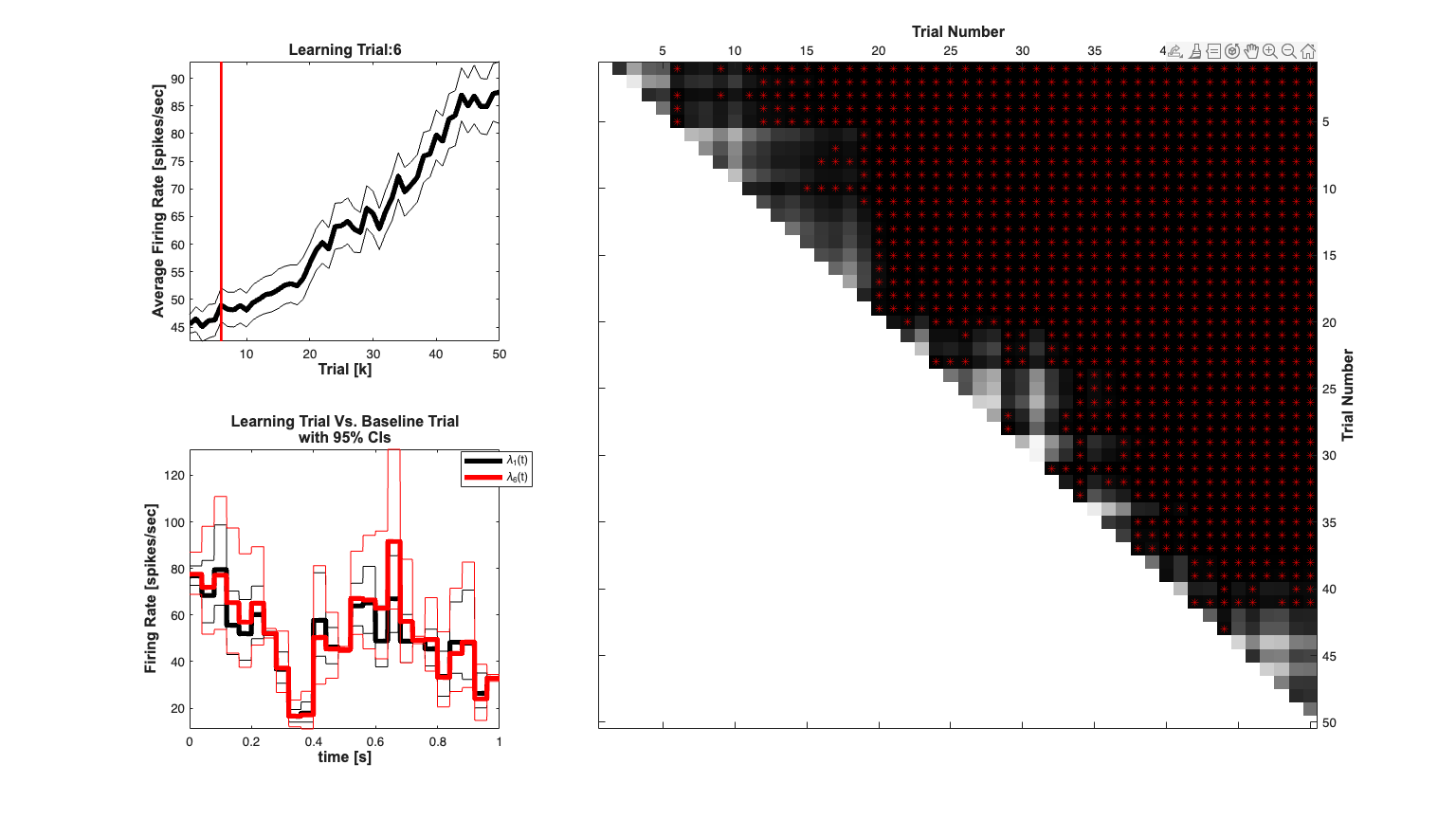
Compare differences across trials
echo off;
close all;
   minTime=0; maxTime = Tmax;
% Generate the basis function so that the estimated effect can be plotted
% at the same temporal resolution as the theoretical effect
 if(~isempty(numBasis))
    basisWidth = (maxTime-minTime)/numBasis;
    sampleRate=1/delta;
    unitPulseBasis=nstColl.generateUnitImpulseBasis(basisWidth,...
        minTime,maxTime,sampleRate);
    basisMat = unitPulseBasis.data;
 end


% close all;

t0=0; tf=Tmax;
[spikeRateBinom, ProbMat,sigMat]=DecodingAlgorithms.computeSpikeRateCIs(xK,...
    WkuFinal,dN,t0,tf,fitType,delta,gammahat,windowTimes);

lt=find(sigMat(1,:)==1,1,'first');
display(['The learning trial (compared to the first trial) is trial #' ...
    num2str(find(sigMat(1,:)==1,1,'first'))]);
scrsz = get(0,'ScreenSize');
h=figure('OuterPosition',[scrsz(3)*.1 scrsz(4)*.1 scrsz(3)*.8 scrsz(4)*.8]);

subplot(2,3,1);
spikeRateBinom.setName(['(' num2str(Tmax) '-0)^-1*\Lambda(0,' ...
    num2str(Tmax) ')']);
spikeRateBinom.plot([],{{' ''k'',''Linewidth'',4'}});
% e = Events(lt,{''});
% e.plot;
v=axis;
plot(lt*[1;1],v(3:4),'r','Linewidth',2);
hx=xlabel('Trial [k]','Interpreter','none'); hold all;
hy=ylabel('Average Firing Rate [spikes/sec]','Interpreter','none');
set([hx, hy],'FontName', 'Arial','FontSize',12,'FontWeight','bold');
title(['Learning Trial:' num2str(lt)],'FontWeight','bold',...
            'Fontsize',12,...
            'FontName','Arial');


h=subplot(2,3,[2 3 5 6]);
K=size(dN,1);
colormap(flipud(gray));
imagesc(ProbMat); hold on;
for k=1:K
    for m=(k+1):K
        if(sigMat(k,m)==1)
            plot3(m,k,1,'r*'); hold on;
        end
    end
end
%
set(h,'XAxisLocation','top','YAxisLocation','right');
hx=xlabel('Trial Number','Interpreter','none'); hold all;
hy=ylabel('Trial Number','Interpreter','none');
set([hx, hy],'FontName', 'Arial','FontSize',12,'FontWeight','bold');

subplot(2,3,4)
stim1 = Covariate(time, basisMat*stimulus(:,1),'Trial1','time','s',...
    'spikes/sec');
temp = ConfidenceInterval(time, basisMat*squeeze(stimCIs(:,1,:)));
stim1.setConfInterval(temp);
stimlt = Covariate(time, basisMat*stimulus(:,lt),'Trial1','time','s',...
    'spikes/sec');
temp = ConfidenceInterval(time, basisMat*squeeze(stimCIs(:,lt,:)));
temp.setColor('r');
stimlt.setConfInterval(temp);
stimltm1 = Covariate(time, basisMat*stimulus(:,lt-1),'Trial1','time','s',...
    'spikes/sec');
temp = ConfidenceInterval(time, basisMat*squeeze(stimCIs(:,lt-1,:)));
temp.setColor('r');
stimltm1.setConfInterval(temp);

% figure;
h1=stim1.plot([],{{' ''k'',''Linewidth'',4'}}); hold all;
h2=stimlt.plot([],{{' ''r'',''Linewidth'',4'}});
hx=xlabel('time [s]','Interpreter','none'); hold all;
hy=ylabel('Firing Rate [spikes/sec]','Interpreter','none');
set([hx, hy],'FontName', 'Arial','FontSize',12,'FontWeight','bold');

title({'Learning Trial Vs. Baseline Trial';'with 95% CIs'},'FontWeight','bold',...
            'Fontsize',12,...
            'FontName','Arial');
h_legend=legend([h1(1) h2(1)],'\lambda_{1}(t)',['\lambda_{' num2str(lt) '}(t)']);
pos = get(h_legend,'position');
set(h_legend, 'position',[pos(1)+.03 pos(2)+.01 pos(3:4)]);
%% Compare differences across trials
echo off;
The learning trial (compared to the first trial) is trial #13
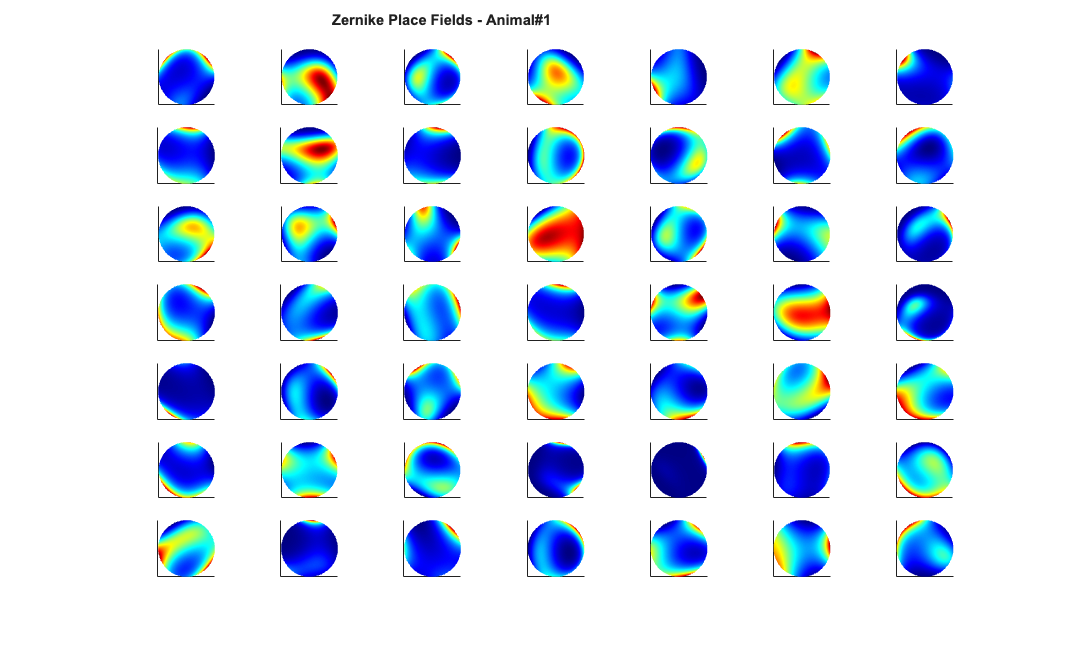
Example 4 - HIPPOCAMPAL PLACE CELL - RECEPTIVE FIELD ESTIMATION
Estimation of receptive fields of neurons is a very common data analysis problem in neuroscience. Here we use the nSTAT software to perform an estimation of the receptive fields of hippocampal place cells using a bivariate Gaussian model and Zernike polynomials. The number of zernike polynomials is based on "An Analysis of Hippocampal Spatio-Temporal Representations Using a Bayesian Algorithm for Neural Spike Train Decoding" Barbieri et. al 2005. The data used herein in was provided by Dr. Ricardo Barbieri on 2/28/2011.
Author: Iahn Cajigas
Date: 3/1/2011
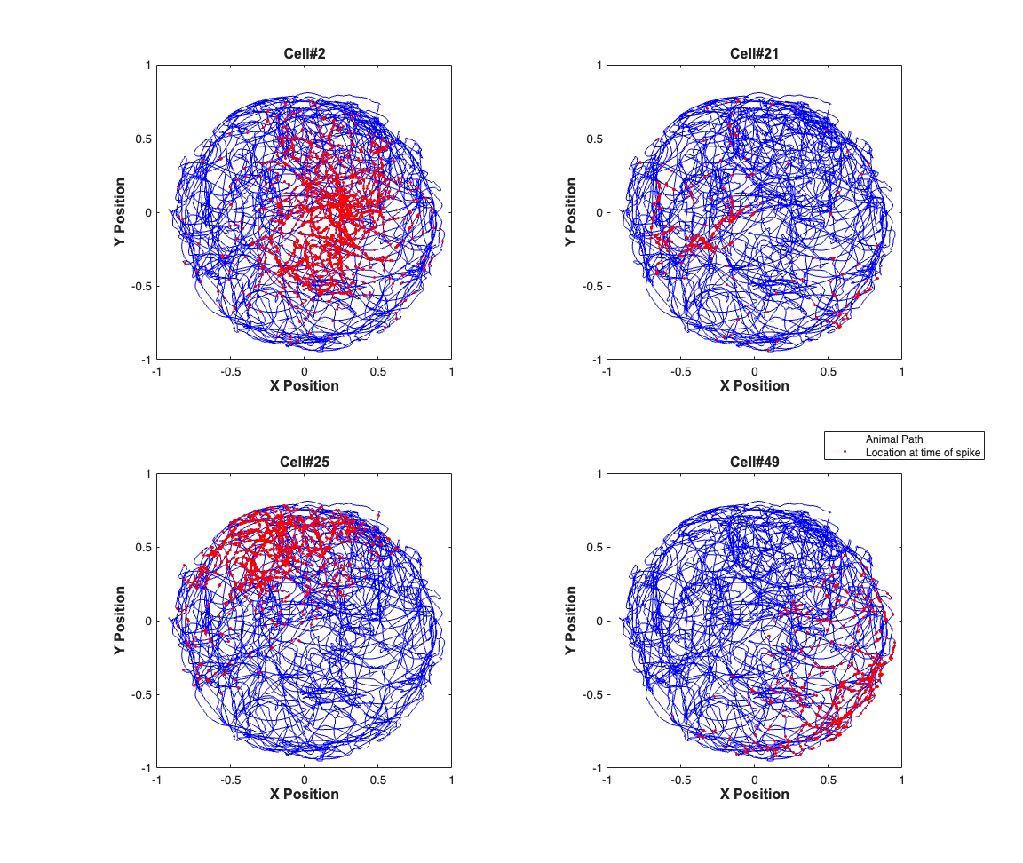
Example Data
The x and y coordinates of a freely foraging rat in a circular environment (70cm in diameter and 30cm high walls) and a fixed visual cue. The x and y coordinates at the time when a spike was observed are marked in red. The position coordinates have been normalized to be between -1 and 1 to allow to simplify the analysis.
    close all;
    load(fullfile(placeCellDataDir,'PlaceCellDataAnimal1.mat'));
    exampleCell = [2 21 25 49];
%     exampleCell = 1:length(neuron);
%     figure(1);
    scrsz = get(0,'ScreenSize');
    h=figure('OuterPosition',[scrsz(3)*.1 scrsz(4)*.1 scrsz(3)*.6 scrsz(4)*.9]);

    for i=1:length(exampleCell)
        subplot(2,2,i);
        h1=plot(x,y,'b','Linewidth',.5); hold on;
        h2=plot(neuron{exampleCell(i)}.xN,neuron{exampleCell(i)}.yN,'r.',...
            'MarkerSize',7);
        hx=xlabel('X Position'); hy=ylabel('Y Position');
%         title(['Animal#1, Cell#' num2str(exampleCell(i))]);
        title(['Cell#' num2str(exampleCell(i))],'FontWeight','bold',...
            'Fontsize',12,'FontName','Arial');
        set([hx, hy],'FontName', 'Arial','FontSize',12,'FontWeight','bold');
        set(gca,'xTick',-1:.5:1,'yTick',-1:.5:1); axis square;
        if(i==4)
            h_legend = legend([h1 h2],'Animal Path',...
                'Location at time of spike');
            pos = get(h_legend,'position');
            set(h_legend, 'position',[pos(1)+.09 pos(2)+.06 pos(3:4)]);
        end
    end
Analyze All Cells
numAnimals=2;
CompilingHelpFile=1;
if(~CompilingHelpFile)
    for n=1:numAnimals
        % load the data
        clear x y neuron time nst tc tcc z;
        load(fullfile(placeCellDataDir,['PlaceCellDataAnimal' num2str(n) '.mat']));

        % Create the spikeTrains for each cell
        for i=1:length(neuron)
            nst{i} = nspikeTrain(neuron{i}.spikeTimes);
        end


        % Convert to polar coordinates
        [theta,r] = cart2pol(x,y);


        % Evaluate the Zernike Polynomials
        % Number of polynomials from "An Analysis of Hippocampal
        % Spatio-Temporal Representations Using a Bayesian Algorithm for Neural
        % Spike Train Decoding" Barbieri et. al 2005
        cnt=0;
        for l=0:3
           for m=-l:l
               if(~any(mod(l-m,2))) % otherwise the polynomial = 0
                cnt = cnt+1;
                z(:,cnt) = zernfun(l,m,r,theta,'norm');
                % zernfun by Paul Fricker
                % http://www.mathworks.com/matlabcentral/fileexchange/7687
               end
           end
        end

        % Data sampled at 30 Hz but just to be sure
        delta=min(diff(time));
        sampleRate = round(1/delta);
        % Define Covariates for the analysis
        baseline = Covariate(time,ones(length(x),1),'Baseline','time','s','',...
                            {'mu'});
        zernike  = Covariate(time,z,'Zernike','time','s','m',{'z1','z2','z3',...
                            'z4','z5','z6','z7','z8','z9','z10'});
        gaussian = Covariate(time,[x y x.^2 y.^2 x.*y],'Gaussian','time',...
                            's','m',{'x','y','x^2','y^2','x*y'});
        covarColl = CovColl({baseline,gaussian,zernike});

        % Create the trial structure
        spikeColl = nstColl(nst);
        trial     = Trial(spikeColl,covarColl);


        % Define how we want to analyze the data
        tc{1} = TrialConfig({{'Baseline','mu'},{'Gaussian',...
                            'x','y','x^2','y^2','x*y'}},sampleRate,[]);
        tc{1}.setName('Gaussian');
        tc{2} = TrialConfig({{'Zernike' 'z1','z2','z3','z4','z5','z6',...
                            'z7','z8','z9','z10'}},sampleRate,[]);
        tc{2}.setName('Zernike');
        tcc = ConfigColl(tc);

        % Perform Analysis (Commented to since data already saved)
         results =Analysis.RunAnalysisForAllNeurons(trial,tcc,0);

        % Save results
            resStruct =FitResult.CellArrayToStructure(results);
            filename = fullfile(dataDir,['PlaceCellAnimal' num2str(n) 'Results']);
            save(filename,'resStruct');
    end
end
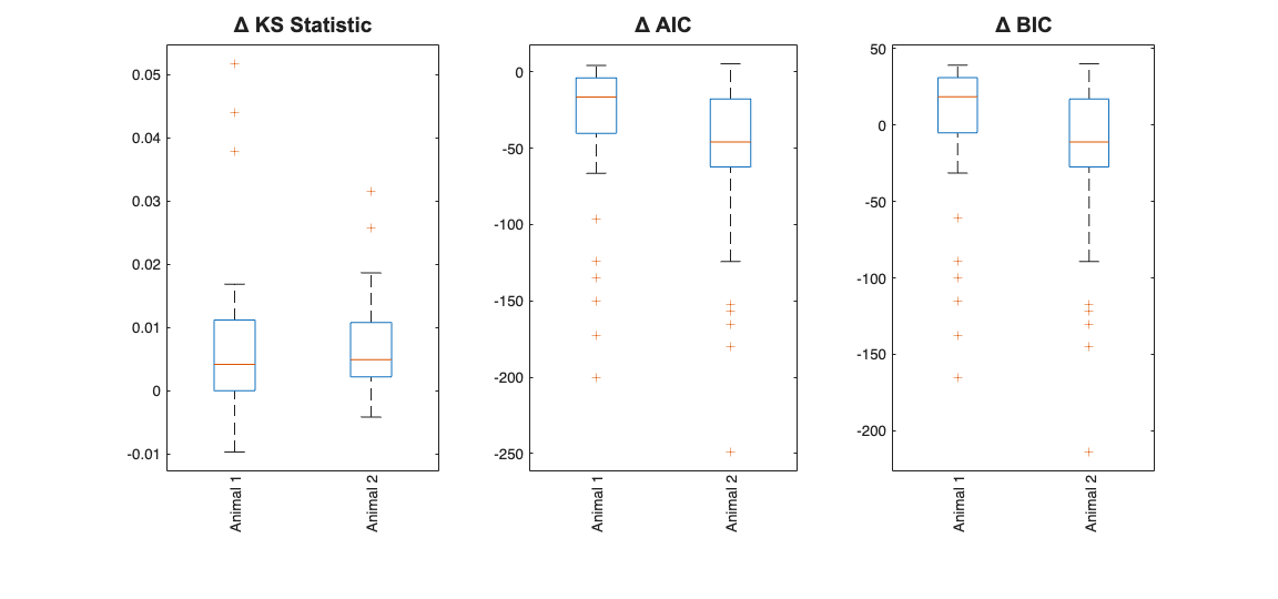
View Summary Statistics
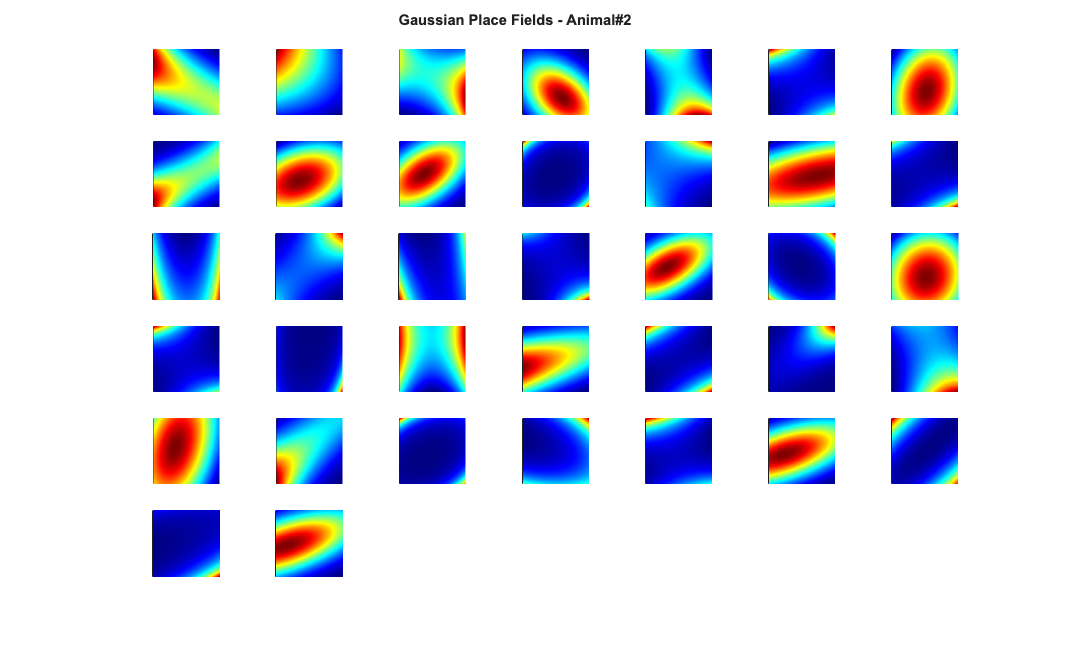
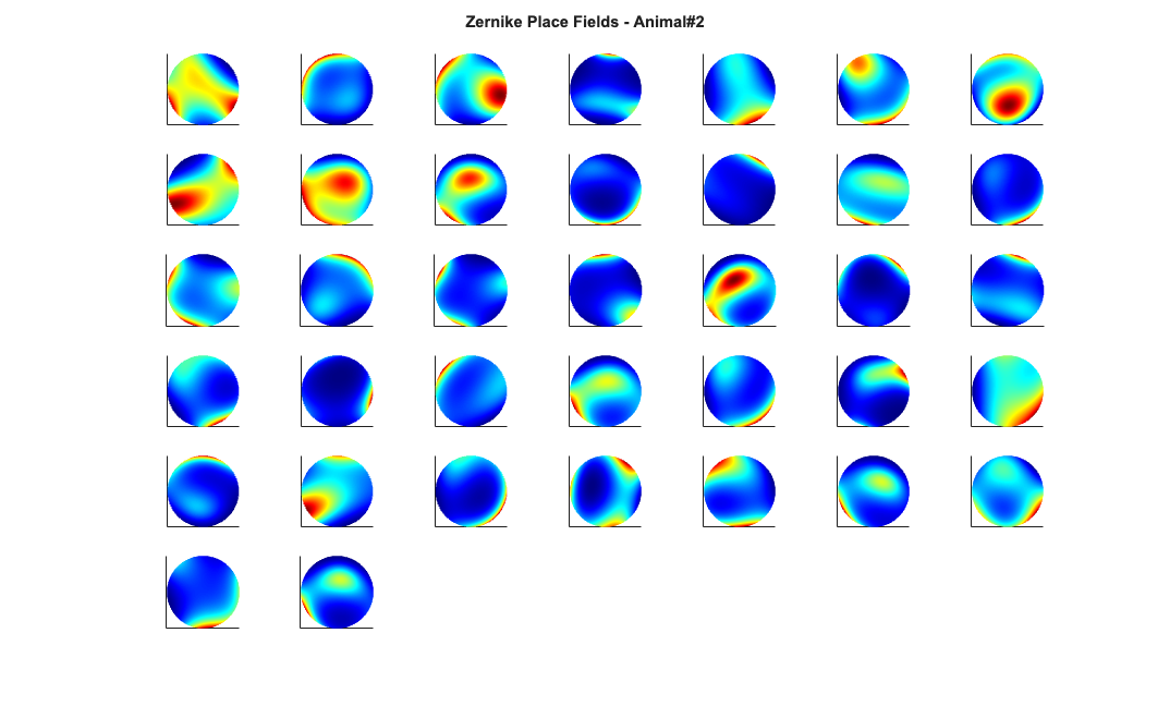
Note the Zernike Polynomials yield better fits in terms of decreased KS Statistics (less deviation from the 45 degree line), reduced AIC and reduced BIC across the majority of cells and for both animals
clear Summary;
numAnimals =2;

for n=1:numAnimals
    resData = load(fullfile(dataDir,['PlaceCellAnimal' num2str(n) 'Results.mat']));
    results = FitResult.fromStructure(resData.resStruct);
    Summary{n} = FitResSummary(results);
%     Summary{n}.plotSummary;
end
close all;
scrsz = get(0,'ScreenSize');
h=figure('OuterPosition',[scrsz(3)*.1 scrsz(4)*.1 scrsz(3)*.6 scrsz(4)*.5]);
subplot(1,3,1);
maxLength = max([Summary{1}.numNeurons,Summary{2}.numNeurons]);
dKS = nan(maxLength, 2);
dKS(1:Summary{1}.numNeurons,1) = (Summary{1}.KSStats(:,1)-Summary{1}.KSStats(:,2)) ;
dKS(1:Summary{2}.numNeurons,2) = (Summary{2}.KSStats(:,1)-Summary{2}.KSStats(:,2)) ;

boxplot(dKS ,{'Animal 1', 'Animal 2'},'labelorientation','inline');
title('\Delta KS Statistic','FontWeight','bold','FontSize',14,...
    'FontName','Arial');


subplot(1,3,2);
dAIC = nan(maxLength, 2);
dAIC(1:Summary{1}.numNeurons,1) = Summary{1}.getDiffAIC(1);
dAIC(1:Summary{2}.numNeurons,2) = Summary{2}.getDiffAIC(1);

boxplot(dAIC ,{'Animal 1', 'Animal 2'},'labelorientation','inline');
title('\Delta AIC','FontWeight','bold','FontSize',14,'FontName','Arial');


subplot(1,3,3);
dBIC = nan(maxLength, 2);
dBIC(1:Summary{1}.numNeurons,1) = Summary{1}.getDiffBIC(1);
dBIC(1:Summary{2}.numNeurons,2) = Summary{2}.getDiffBIC(1);

boxplot(dBIC ,{'Animal 1', 'Animal 2'},'labelorientation','inline'); %ylabel('\Delta BIC'); %xticklabel_rotate([],45,[],'Fontsize',6);
title('\Delta BIC','FontWeight','bold','FontSize',14,'FontName','Arial');

%  close all;
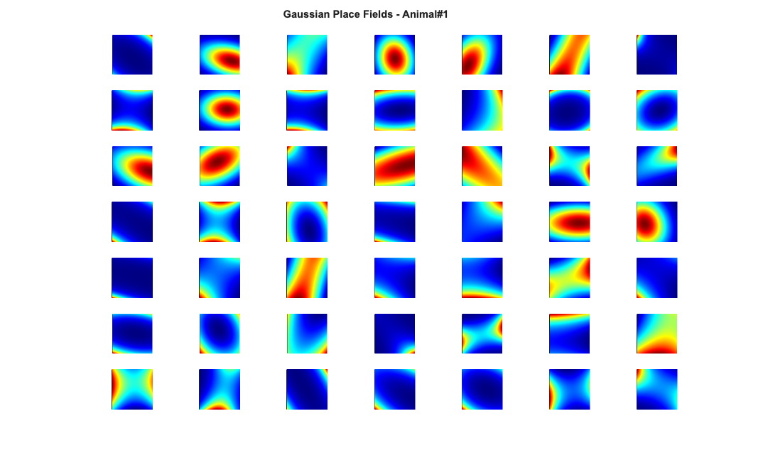
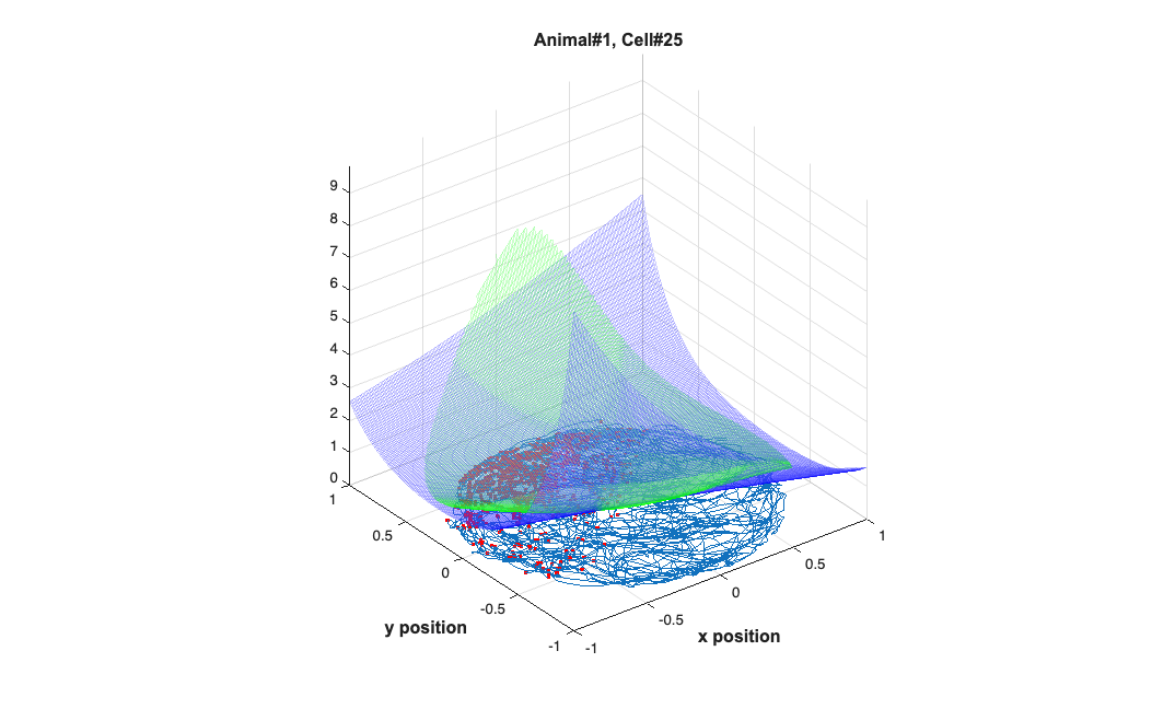
Visualize the results
close all;
% Define a grid
[x_new,y_new]=meshgrid(-1:.01:1); %define new x and y
y_new = flipud(y_new); x_new = fliplr(x_new);
[theta_new,r_new] = cart2pol(x_new,y_new);

%Data for the gaussian fit
newData{1} =ones(size(x_new));
newData{2} =x_new; newData{3} =y_new;
newData{4} =x_new.^2; newData{5} =y_new.^2;
newData{6} =x_new.*y_new;


% Zernike polynomials only defined on the unit disk
idx = r_new<=1;
zpoly = cell(1,10);
cnt=0;
for l=0:3
   for m=-l:l
       if(~any(mod(l-m,2)))
        cnt = cnt+1;
        temp = nan(size(x_new));
        temp(idx) = zernfun(l,m,r_new(idx),theta_new(idx),'norm');
        zpoly{cnt} = temp;
       end
   end
end


for n=1:numAnimals

    clear lambdaGaussian lambdaZernike;
    load(fullfile(placeCellDataDir,['PlaceCellDataAnimal' num2str(n) '.mat']));
    resData = load(fullfile(dataDir,['PlaceCellAnimal' num2str(n) 'Results.mat']));
    results = FitResult.fromStructure(resData.resStruct);

    for i=1:length(neuron)
        % Evaluate our fits using the new data and the estimated parameters
        lambdaGaussian{i} = results{i}.evalLambda(1,newData);
        lambdaZernike{i} =  results{i}.evalLambda(2,zpoly);
    end


    % Plot the receptive fields
    for i=1:length(neuron)
        % 3d plot of an example place field


        % 2d plot of all the cell's fields
        if(n==1)
            h4=figure(4);
            colormap('jet');
            if(i==1)
                tb=annotation(h4,'textbox',...
                    [0.283261904761904 0.928571428571418 ...
                    0.392857142857143 0.0595238095238095],...
                    'String',{['Gaussian Place Fields - Animal#' ...
                    num2str(n)]},'FitBoxToText','on','Fontsize',11,...
                    'FontName','Arial','FontWeight','bold','LineStyle',...
                    'none','HorizontalAlignment','center'); hold on;
            end
            subplot(7,7,i);
        elseif(n==2)
            h6=figure(6);
            colormap('jet');
            if(i==1)
                annotation(h6,'textbox',...
                    [0.283261904761904 0.928571428571418 ...
                    0.392857142857143 0.0595238095238095],...
                    'String',{['Gaussian Place Fields - Animal#' ...
                    num2str(n)]},'FitBoxToText','on','Fontsize',11,...
                    'FontName','Arial','FontWeight','bold','LineStyle',...
                    'none','HorizontalAlignment','center'); hold on;
            end
            subplot(6,7,i);
        end
        pcolor(x_new,y_new,lambdaGaussian{i}), shading interp
        axis square; set(gca,'xtick',[],'ytick',[]);
        set(gca, 'Box'         , 'off');

        if(n==1)
            h5=figure(5);
            colormap('jet');
            if(i==1)
                annotation(h5,'textbox',...
                    [0.303261904761904 0.928571428571418 ...
                    0.392857142857143 0.0595238095238095],...
                    'String',{['Zernike Place Fields - Animal#' ...
                    num2str(n)]},'FitBoxToText','on','Fontsize',11,...
                    'FontName','Arial','FontWeight','bold','LineStyle','none'); hold on;

            end
            subplot(7,7,i);
        elseif(n==2)
            h7=figure(7);
            colormap('jet');
            if(i==1)
               annotation(h7,'textbox',...
                    [0.303261904761904 0.928571428571418 ...
                    0.392857142857143 0.0595238095238095],...
                    'String',{['Zernike Place Fields - Animal#' ...
                    num2str(n)]},'FitBoxToText','on','Fontsize',11,...
                    'FontName','Arial','FontWeight','bold','LineStyle',...
                    'none','HorizontalAlignment','center'); hold on;
            end
            subplot(6,7,i);
        end
        pcolor(x_new,y_new,lambdaZernike{i}), shading interp
        axis square;
        set(gca,'xtick',[],'ytick',[]);
        set(gca, 'Box'         , 'off');
    end


end
    clear lambdaGaussian lambdaZernike;
    load(fullfile(placeCellDataDir,'PlaceCellDataAnimal1.mat'));
    resData = load(fullfile(dataDir,'PlaceCellAnimal1Results.mat'));
    results = FitResult.fromStructure(resData.resStruct);

    for i=1:length(neuron)
        % Evaluate our fits using the new data and the estimated parameters
        lambdaGaussian{i} = results{i}.evalLambda(1,newData);
        lambdaZernike{i} =  results{i}.evalLambda(2,zpoly);
    end


%     h1=plot(x,y,'b');
%     h2=plot(x,y,'g');
    %
    exampleCell = 25;
%     figure(8);
%     plot(x,y,'b',neuron{exampleCell}.xN,neuron{exampleCell}.yN,'r.');
%     xlabel('x'); ylabel('y');
%     title(['Animal#1, Cell#' num2str(exampleCell)]);
%
    close all;
    h9=figure(9);
    h_mesh = mesh(x_new,y_new,lambdaGaussian{exampleCell},'AlphaData',0);
    get(h_mesh,'AlphaData');
    set(h_mesh,'FaceAlpha',0.2,'EdgeAlpha',0.2,'EdgeColor','b');
    hold on;
    h_mesh = mesh(x_new,y_new,lambdaZernike{exampleCell},'AlphaData',0);
    get(h_mesh,'AlphaData');
    set(h_mesh,'FaceAlpha',0.2,'EdgeAlpha',0.2,'EdgeColor','g');


%     h_legend=legend('\lambda_{Gaussian}','\lambda_{Zernike}');
%     set(h_legend,'FontSize',20);
    plot(x,y,neuron{exampleCell}.xN,neuron{exampleCell}.yN,'r.');
    axis tight square;
    xlabel('x position'); ylabel('y position');
    title(['Animal#1, Cell#' num2str(exampleCell)],'FontWeight','bold',...
        'Fontsize',12,'FontName','Arial');
    hx=get(gca,'XLabel');  hy=get(gca,'YLabel');
    set([hx, hy],'FontName', 'Arial','FontSize',12,'FontWeight','bold');
Example 5 - STIMULUS DECODING
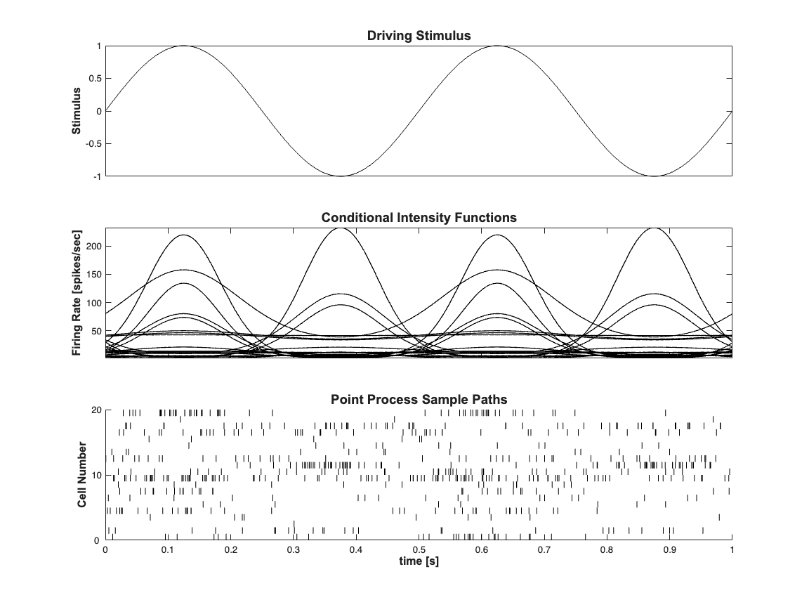
In this example we show how to decode a univariate and a bivariate stimulus based on a point process observations using nSTAT. Even though due to the simulated nature of the data, we know the exact condition intensity function, we estimate the parameters before moving on to the decoding stage.
Generate the conditional Intensity Function
    close all; clear all;
    [dataDir,mEPSCDir,explicitStimulusDir,psthDir,placeCellDataDir] = ...
        getPaperDataDirs();
    delta = 0.001; Tmax = 1;
    time = 0:delta:Tmax;
    numRealizations = 20;
    f=2; b1=randn(numRealizations,1);b0=log(10*delta)+randn(numRealizations,1);
    x = sin(2*pi*f*time);
    clear nst;
    for i=1:numRealizations
        expData = exp(b1(i)*x+b0(i));
        lambdaData = expData./(1+expData);

        if(i==1)
            lambda = Covariate(time,lambdaData./delta, ...
                '\Lambda(t)','time','s','spikes/sec',{'\lambda_{1}'},...
                {{' ''b'', ''LineWidth'' ,2'}});
        else
            tempLambda = Covariate(time,lambdaData./delta, ...
                '\Lambda(t)','time','s','spikes/sec',{'\lambda_{1}'},...
                {{' ''b'', ''LineWidth'' ,2'}});
            lambda = lambda.merge(tempLambda);
        end

        spikeColl = CIF.simulateCIFByThinningFromLambda(...
            lambda.getSubSignal(i),1);
        nst{i} = spikeColl.getNST(1);
    end
        spikeColl = nstColl(nst);scrsz = get(0,'ScreenSize');
        h=figure('Position',[scrsz(3)*.1 scrsz(4)*.1 ...
            scrsz(3)*.6 scrsz(4)*.8]);
%         figure;
        subplot(3,1,1); plot(time,x,'k');
        set(gca,'xtick',[],'xtickLabel',[]); ylabel('Stimulus');
            hx=get(gca,'XLabel');  hy=get(gca,'YLabel');
            set([hx, hy],'FontName', 'Arial','FontSize',12,'FontWeight','bold');
            title('Driving Stimulus','FontWeight','bold',...
                'FontSize',14,'FontName','Arial');
        subplot(3,1,2); lambda.plot([],{{' ''k'',''Linewidth'',1'}});
            legend off;
            hy=ylabel('Firing Rate [spikes/sec]', 'Interpreter','none');
            hx=xlabel('','Interpreter','none');
            set([hx, hy],'FontName', 'Arial','FontSize',12,...
                'FontWeight','bold');
            set(gca,'xtickLabel',[]);
            title('Conditional Intensity Functions','FontWeight',...
                'bold','FontSize',14,'FontName','Arial');

        subplot(3,1,3); spikeColl.plot;
            set(gca,'ytick',0:10:numRealizations,'ytickLabel',...
                0:10:numRealizations);
            xlabel('time [s]','Interpreter','none');
            ylabel('Cell Number','Interpreter','none');
            hx=get(gca,'XLabel');  hy=get(gca,'YLabel');
            set([hx, hy],'FontName', 'Arial','FontSize',12,'FontWeight','bold');
            title('Point Process Sample Paths','FontWeight',...
                'bold','FontSize',14,'FontName','Arial');

stim = Covariate(time,sin(2*pi*f*time),'Stimulus','time','s','V',{'stim'});
baseline = Covariate(time,ones(length(time),1),'Baseline','time','s','',...
                    {'constant'});

%     close all;
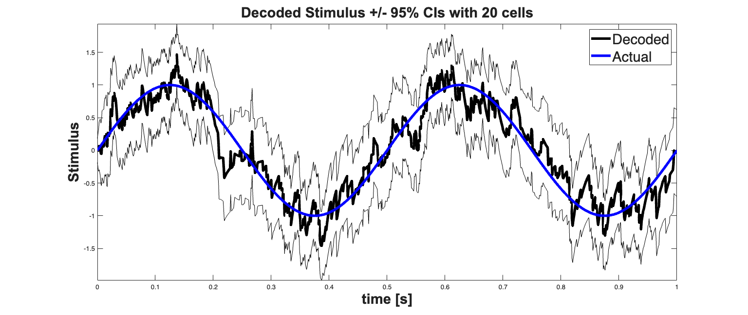
close all;

clear lambdaCIF;
spikeColl.resample(1/delta);
dN=spikeColl.dataToMatrix;

% Make noise according to the dynamic range of the stimulus
Q=std(stim.data(2:end)-stim.data(1:end-1));
Px0=.1; A=1;
x0 = x(:,1); yT=x(:,end);
Pi0 = eps*eye(size(x0,1),size(x0,1));
PiT = eps*eye(size(x0,1),size(x0,1));


[x_p, W_p, x_u, W_u] = nstat.decoding.PPAF.PPDecodeFilterLinear(A, ...
    Q, dN',b0,b1','binomial',delta);
%
h=figure('Position',[scrsz(3)*.1 scrsz(4)*.1 scrsz(3)*.8 scrsz(4)*.6]);
zVal=1.96;
ciLower = min(x_u(1:end)-zVal*sqrt(squeeze(W_u(1:end)))',...
    x_u(1:end)+zVal*sqrt(squeeze(W_u(1:end))'));
ciUpper = max(x_u(1:end)-zVal*sqrt(squeeze(W_u(1:end)))',...
    x_u(1:end)+zVal*sqrt(squeeze(W_u(1:end))'));

estimatedStimulus = Covariate(time,x_u(1:end),'\hat{x}(t)','time','s','');
CI= ConfidenceInterval(time,[ciLower', ciUpper'],'\hat{x}(t)','time','s','');
estimatedStimulus.setConfInterval(CI);

% hold all;
% hEst=plot(time,x_u(1:end),'b','Linewidth',2); hold on;
% plot(time, [ciUpper', ciLower'],'b');

hEst = estimatedStimulus.plot([],{{' ''k'',''Linewidth'',4'}});
hStim=stim.plot([],{{' ''b'',''Linewidth'',4'}});
legend off;
h_legend=legend([hEst(1) hStim],'Decoded','Actual');
set(h_legend,'Interpreter','none');
set(h_legend,'FontSize',22);
title(['Decoded Stimulus +/- 95% CIs with ' num2str(numRealizations) ' cells'],...
    'FontWeight','bold','Fontsize',22,'FontName','Arial');
xlabel('time [s]','Interpreter','none');
ylabel('Stimulus','Interpreter','none');
hx=get(gca,'XLabel');  hy=get(gca,'YLabel');
set([hx, hy],'FontName', 'Arial','FontSize',22,'FontWeight','bold');
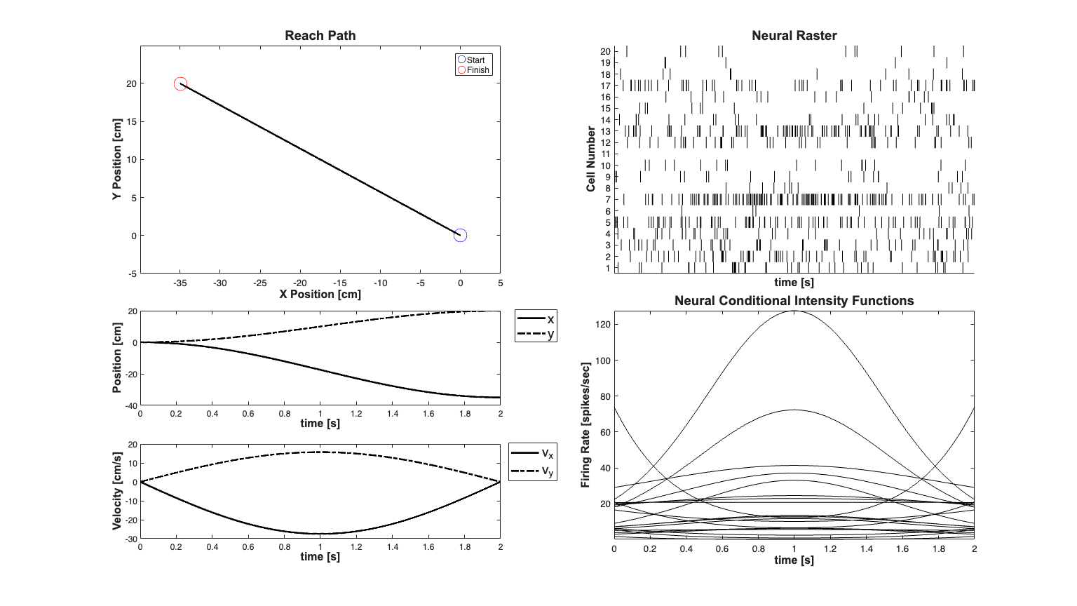
Example 5b - Arm reaching to target Simulation
See L. Srinivasan, U. T. Eden, A. S. Willsky, and E. N. Brown, "A state-space analysis for reconstruction of goal-directed movements using neural signals.," Neural computation, vol. 18, no. 10, pp. 2465?2494, Oct. 2006.
    close all;
    clear all;
    [dataDir,mEPSCDir,explicitStimulusDir,psthDir,placeCellDataDir] = ...
        getPaperDataDirs();
    %Process noise covariance only drives the movement velocity
    q=1e-4;
    Q=diag([1e-12 1e-12 q q]);

    delta = .001;        % Time increment
    r=1e-6;   % in meters^2
    p=1e-6;    % in meters^2/s^2
    PiT=diag([r r p p]); % Uncertainty in the target state
    Pi0=PiT;
    T=2;                 % Reach Duration

    x0 = [0;0;0;0];     % Initial Position and velocities (states)
    xT = [-.35;.2; 0;0];% Final Target
    time=0:delta:T;     % time vector

    A=[1 0 delta 0    ; %State transition matrix
       0 1 0     delta;
       0 0 1     0    ;
       0 0 0     1    ];

    x=zeros(4,length(time));


% Simulate a reach trajectory
% Differs from reference by multiplication by delta instead of division so
% that the velocity has units of meters per second
    R=chol(Q);
    L=chol(PiT);
    for k=1:length(time)
        if(k==1)
            x(:,k)=x0;
        else
             x(:,k)=A*x(:,k-1)+...
                 delta/(2)*(pi/T)^2*cos(pi*time(k)/T)*[0;0;...
                 xT(1)-x0(1);xT(2)-x0(2)]; %Reach to target model
            %x(:,k)=A*x(:,k-1)+R*randn(size(x,1),1); %Random walk model
        end

    end
    xT =x(:,end); % The target generated by the model
    yT=xT;        % Assume we have observed the actual target position with uncertainty PiT

    %Define Q according to the dynamic range of the movement above
    Q=diag(var(diff(x,[],2),[],2))*100;

    % Plot the movement trajectories and the hand path
    scrsz = get(0,'ScreenSize');
    fig1=figure('OuterPosition',[scrsz(3)*.1 scrsz(4)*.1 ...
        scrsz(3)*.8 scrsz(4)*.8]);
    %Plot The movement path
    subplot(4,2,[1 3]);
    plot(100*x(1,:),100*x(2,:),'k','Linewidth',2);
    xlabel('X Position [cm]'); ylabel('Y Position [cm]');
    hx=get(gca,'XLabel');  hy=get(gca,'YLabel');
    set([hx, hy],'FontName', 'Arial','FontSize',12,'FontWeight','bold');
    title('Reach Path','FontWeight','bold','Fontsize',14,'FontName','Arial');
    hold on;
    axis([sort([100*x0(1)+5, 100*xT(1)-5]), sort([100*x0(2)-5, 100*xT(2)+5])]);
    h1=plot(100*x(1,1),100*x(2,1),'bo','MarkerSize',14);
    h2=plot(100*x(1,end),100*x(2,end),'ro','MarkerSize',14);
    legend([h1 h2],'Start','Finish','Location','NorthEast');


    subplot(4,2,5); h1=plot(time,100*x(1,:),'k','Linewidth',2); hold on;
    h2=plot(time,100*x(2,:),'k-.','Linewidth',2);
    h_legend=legend([h1,h2],'x','y','Location','NorthEast');
    set(h_legend,'FontSize',14)
    pos = get(h_legend,'position');
    set(h_legend, 'position',[pos(1)+.06 pos(2)+.01 pos(3:4)]);
    hx=xlabel('time [s]'); hy=ylabel('Position [cm]');
    set([hx, hy],'FontName', 'Arial','FontSize',12,'FontWeight','bold');
    % Plot the velocity profiles

    subplot(4,2,7);
    h1=plot(time,100*x(3,:),'k','Linewidth',2); hold on;
    h2=plot(time,100*x(4,:),'k-.','Linewidth',2);
    h_legend=legend([h1 h2],'v_x','v_y','Location','NorthEast');
    xlabel('time [s]');
    set(h_legend,'FontSize',14);
    pos = get(h_legend,'position');
    set(h_legend, 'position',[pos(1)+.06 pos(2)+.01 pos(3:4)]);
    hx=xlabel('time [s]'); hy=ylabel('Velocity [cm/s]');
    set([hx, hy],'FontName', 'Arial','FontSize',12,'FontWeight','bold');
    %

    gamma=0;
    windowTimes=[0, 0.001];


% Simulate neural responses
    % logit(lambda_i*delta) = mu_i + b_x_i*v_x + b_y_i*v_y
    % logit(lambda_i*delta) = X_i*beta_i;
    numCells = 20;
    bCoeffs=10*(rand(numCells,2)-.5);           % b_i = [b_x_i b_y_i] ~ U(-5, 5);
    phiMax = atan2(bCoeffs(:,2),bCoeffs(:,1));  % Maximal firing direction of cell
    phiMaxNorm = (phiMax+pi)./(2*pi);
    meanMu = log(10*delta); % baseline firing rate -10Hz
    MuCoeffs = meanMu+randn(numCells,1);   % mu_i ~ G(meanMu,1)

    dataMat = [ones(length(time),1) x(3,:)' x(4,:)']; % design matrix: X (
    coeffs = [MuCoeffs bCoeffs]; % coefficient vector: beta
    fitType='binomial';
    clear nst;
    for i=1:numCells
         tempData  = exp(dataMat*coeffs(i,:)');

         if(strcmp(fitType,'poisson'))
             lambdaData = tempData;
         else
            lambdaData = tempData./(1+tempData); % Conditional Intensity Function for ith cell
         end
         lambda{i}=Covariate(time,lambdaData./delta, ...
             '\Lambda(t)','time','s','spikes/sec',...
             {strcat('\lambda_{',num2str(i),'}')},{{' ''b'' '}});
         lambda{i}=lambda{i}.resample(1/delta);

         % Generate CIF representation in case we want to use the symbolic
         % versions of the PPDecodeFilter (i.e. not PPDecodeFilterLinear
         lambdaCIF{i} = CIF([MuCoeffs(i) 0 0 bCoeffs(i,:)],...
             {'one','x','y','vx','vy'},{'x','y','vx','vy'},fitType);
         % generate one realization for each cell
         tempSpikeColl{i} = CIF.simulateCIFByThinningFromLambda(lambda{i},1);          nst{i} = tempSpikeColl{i}.getNST(1);     % grab the realization
         nst{i}.setName(num2str(i));              % give each cell a unique name
         subplot(4,2,[6 8]);
         h2=lambda{i}.plot([],{{' ''k'', ''LineWidth'' ,.5'}});
         legend off; hold all; % Plot the CIF


    end
    title('Neural Conditional Intensity Functions','FontWeight',...
        'bold','Fontsize',14,'FontName','Arial');
    hx=xlabel('time [s]','Interpreter','none');
    hy=ylabel('Firing Rate [spikes/sec]','Interpreter','none');
    set([hx, hy],'FontName', 'Arial','FontSize',12,'FontWeight','bold');
    spikeColl = nstColl(nst); % Create a neural spike train collection

    subplot(4,2,[2,4]); spikeColl.plot;
    set(gca,'xtick',[],'xtickLabel',[]);
    title('Neural Raster','FontWeight','bold','Fontsize',14,...
        'FontName','Arial');
    hx=xlabel('time [s]','Interpreter','none');
    hy=ylabel('Cell Number','Interpreter','none');
    set([hx, hy],'FontName', 'Arial','FontSize',12,'FontWeight','bold');

%     close all;
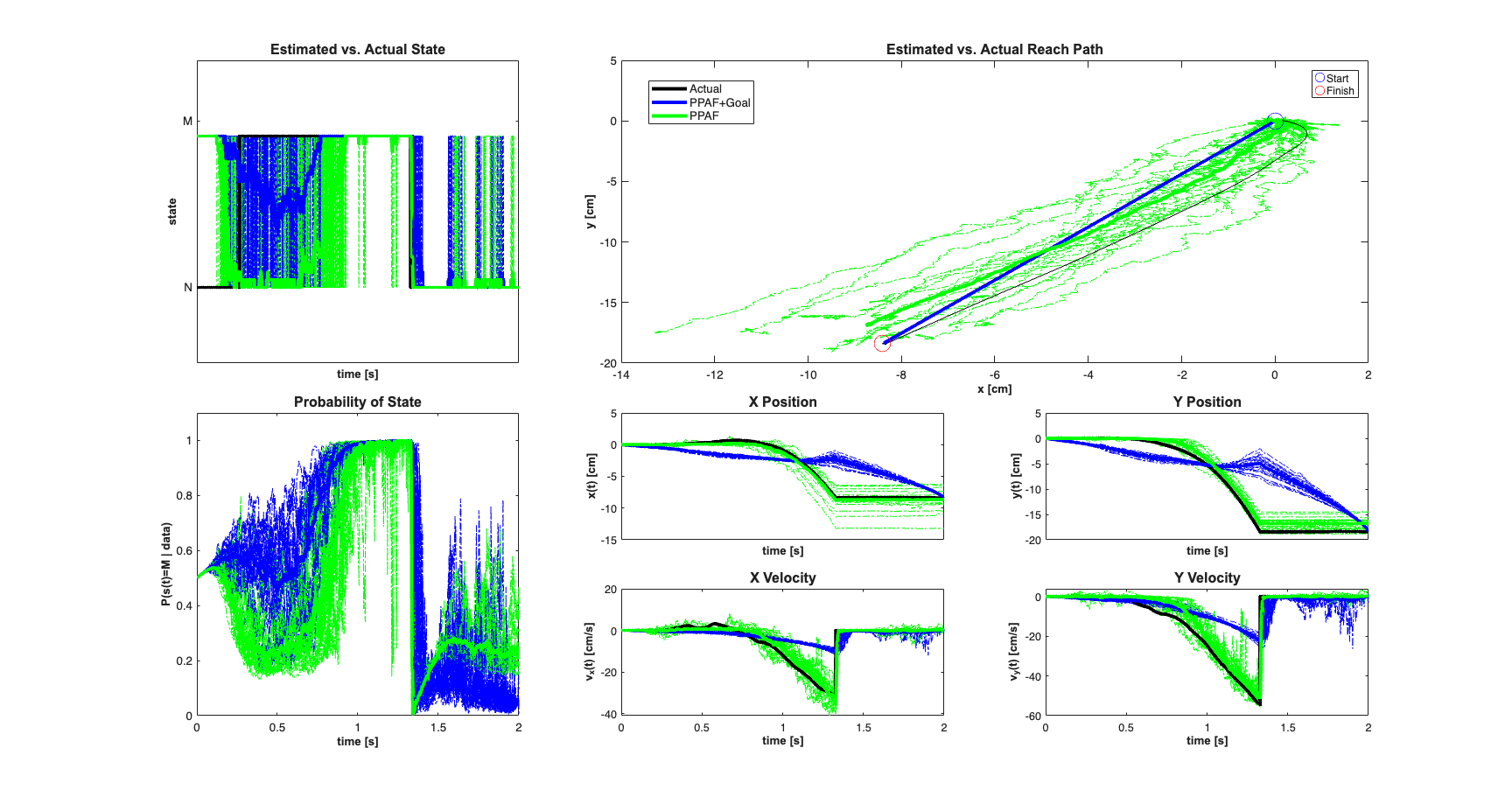
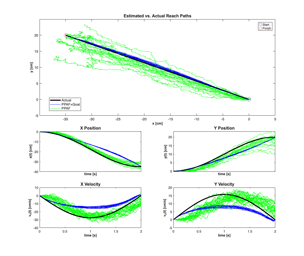
close all;
numExamples=20;
scrsz = get(0,'ScreenSize');
fig1=figure('OuterPosition',[scrsz(3)*.1 scrsz(4)*.1 ...
    scrsz(3)*.6 scrsz(4)*.9]);
for k=1:numExamples
     bCoeffs=10*(rand(numCells,2)-.5);           % b_i = [b_x_i b_y_i] ~ U(-5, 5);
    phiMax = atan2(bCoeffs(:,2),bCoeffs(:,1));  % Maximal firing direction of cell
    phiMaxNorm = (phiMax+pi)./(2*pi);
    meanMu = log(10*delta);  % baseline firing rate
    MuCoeffs = meanMu+randn(numCells,1);   % mu_i ~ G(meanMu,1)

    dataMat = [ones(length(time),1) x(3,:)' x(4,:)']; % design matrix: X (
    coeffs = [MuCoeffs bCoeffs]; % coefficient vector: beta
    fitType='binomial';
    clear nst lambda;


    for i=1:numCells
        tempData  = exp(dataMat*coeffs(i,:)');
         if(strcmp(fitType,'poisson'))
            lambdaData = tempData;
         else
             % Conditional Intensity Function for ith cell
            lambdaData = tempData./(1+tempData);
         end
         lambda{i}=Covariate(time,lambdaData./delta, ...
             '\Lambda(t)','time','s','spikes/sec',...
             {strcat('\lambda_{',num2str(i),'}')},{{' ''b'' '}});
         lambda{i}=lambda{i}.resample(1/delta);

         % Generate CIF representation in case we want to use the symbolic
         % versions of the PPDecodeFilter (i.e. not PPDecodeFilterLinear
         % generate one realization for each cell
         tempSpikeColl{i} = CIF.simulateCIFByThinningFromLambda(lambda{i},1);
         nst{i} = tempSpikeColl{i}.getNST(1);     % grab the realization
         nst{i}.setName(num2str(i));              % give each cell a unique name

    end

    % Plot the neural raster across all the cells
    spikeColl = nstColl(nst); % Create a neural spike train collection

    % Based on the temporal resolution defined by delta, bin the data and get
    % a matrix representation of the neural firing
    dN=spikeColl.dataToMatrix';
    dN(dN>1)=1; % more than one spike per bin will be treated as one spike. In
                % general we should pick delta small enough so that there is
                % only one spike per bin

    [C,N]   = size(dN); % N time samples, C cells

    beta=[zeros(2,numCells);  bCoeffs'];


    %Use the Goal Directed Movement Version of the Point Process adaptive
    %Filter
    [x_p, W_p, x_u, W_u,x_uT,W_uT,x_pT,W_pT] = ...
        nstat.decoding.PPAF.PPDecodeFilterLinear(A, Q, dN,...
        MuCoeffs,beta,fitType,delta,gamma,windowTimes,x0, Pi0, yT,PiT,0);

    %Use the Free Movement Version of the Point Process adaptive
    %Filter
    [x_pf, W_pf, x_uf, W_uf] = ...
        nstat.decoding.PPAF.PPDecodeFilterLinear(A, Q, dN,...
        MuCoeffs,beta,fitType,delta,gamma,windowTimes,x0);


    if(k==numExamples)
        subplot(4,2,1:4);h1=plot(100*x(1,:),100*x(2,:),'k','LineWidth',3);
        hold on;
        axis([sort([100*x0(1)+5, 100*xT(1)-5]), ...
            sort([100*x0(2)-5, 100*xT(2)+5])]);
        title('Estimated vs. Actual Reach Paths',...
            'FontWeight','bold','Fontsize',12,'FontName','Arial');
    end
    subplot(4,2,1:4);h2=plot(100*x_u(1,:)',100*x_u(2,:)','b'); hold all;
    subplot(4,2,1:4);h3=plot(100*x_uf(1,:)',100*x_uf(2,:)','g');
    hx=xlabel('x [cm]'); hy=ylabel('y [cm]');
    set([hx, hy],'FontName', 'Arial','FontSize',10,'FontWeight','bold');
    h1=plot(100*x0(1),100*x0(2),'bo','MarkerSize',10); hold on;
    h2=plot(100*xT(1),100*xT(2),'ro','MarkerSize',10);
    legend([h1 h2],'Start','Finish','Location','NorthEast');


    subplot(4,2,5);
    h1=plot(time,100*x(1,:),'k','LineWidth',3); hold on;
    h2=plot(time,100*x_u(1,:)','b');
    h3=plot(time,100*x_uf(1,:)','g');
    hy=ylabel('x(t) [cm]'); hx=xlabel('time [s]');
    set(gca,'xtick',[],'xtickLabel',[]);
    set([hx, hy],'FontName', 'Arial','FontSize',10,'FontWeight','bold');
    title('X Position','FontWeight','bold','Fontsize',12,'FontName','Arial');

    subplot(4,2,6);
    h1=plot(time,100*x(2,:),'k','LineWidth',3); hold on;
    h2=plot(time,100*x_u(2,:)','b');
    h3=plot(time,100*x_uf(2,:)','g');
    h_legend=legend([h1(1) h2(1) h3(1)],'Actual','PPAF+Goal',...
        'PPAF','Location','SouthEast');
    hy=ylabel('y(t) [cm]'); hx=xlabel('time [s]');
    set(gca,'xtick',[],'xtickLabel',[]);
    set([hx, hy],'FontName', 'Arial','FontSize',10,'FontWeight','bold');
    title('Y Position','FontWeight','bold','Fontsize',12,'FontName','Arial');
    set(h_legend,'FontSize',10)
    pos = get(h_legend,'position');
    set(h_legend, 'position',[pos(1)-.63 pos(2)+.23 pos(3:4)]);

    subplot(4,2,7);
    h1=plot(time,100*x(3,:),'k','LineWidth',3); hold on;
    h2=plot(time,100*x_u(3,:)','b');
    h3=plot(time,100*x_uf(3,:)','g');
    hy=ylabel('v_{x}(t) [cm/s]'); hx=xlabel('time [s]');
    set([hx, hy],'FontName', 'Arial','FontSize',10,'FontWeight','bold');
    title('X Velocity','FontWeight','bold','Fontsize',12,'FontName','Arial');

    subplot(4,2,8);
    h1=plot(time,100*x(4,:),'k','LineWidth',3); hold on;
    h2=plot(time,100*x_u(4,:)','b');
    h3=plot(time,100*x_uf(4,:)','g');
    hy=ylabel('v_{y}(t) [cm/s]'); hx=xlabel('time [s]');
    set([hx, hy],'FontName', 'Arial','FontSize',10,'FontWeight','bold');
    title('Y Velocity','FontWeight','bold','Fontsize',12,'FontName','Arial');


end

%     close all;
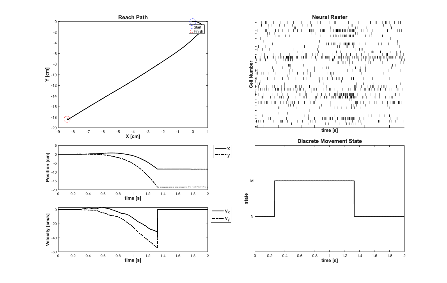
Experiment 6 - Hybrid Point Process Filter Example
NOTE THIS EXAMPLE WAS NOT INCLUDED IN THE FINAL VERSION OF THE PAPER This example is based on an implementation of the Hybrid Point Process filter described in General-purpose filter design for neural prosthetic devices by Srinivasan L, Eden UT, Mitter SK, Brown EN in J Neurophysiol. 2007 Oct, 98(4):2456-75.
Problem Statement
Suppose that a process of interest can be modeled as consisting of several discrete states where the evolution of the system under each state can be modeled as a linear state space model. The observations of both the state and the continuous dynamics are not direct, but rather observed through how the continuous and discrete states affect the firing of a population of neurons. The goal of the hybrid filter is to estimate both the continuous dynamics and the underlying system state from only the neural population firing (point process observations).
To illustrate the use of this filter, we consider a reaching task. We assume two underlying system states s=1="Not Moving"=NM and s=2="Moving"=M. Under the "Not Moving" the position of the arm remain constant, whereas in the "Moving" state, the position and velocities evolved based on the arm acceleration that is modeled as a gaussian white noise process.
Under both the "Moving" and "Not Moving" states, the arm evolution state vector is
![$${\bf{x}} = {[x,y,{v_x},{v_y},{a_x},{a_y}]^T}$$](nSTATPaperExamples_eq12496553100641641814.png)
Generated Simulated Arm Reach
clear all;
[dataDir,mEPSCDir,explicitStimulusDir,psthDir,placeCellDataDir] = ...
    getPaperDataDirs();
close all;
delta=0.001;
Tmax=2;
time=0:delta:Tmax;
A{2} = [1 0 delta 0     delta^2/2   0;
        0 1 0     delta 0           delta^2/2;
        0 0 1     0     delta       0;
        0 0 0     1     0           delta;
        0 0 0     0     1           0;
        0 0 0     0     0           1];

A{1} = [1 0 0 0 0 0;
        0 1 0 0 0 0;
        0 0 0 0 0 0;
        0 0 0 0 0 0;
        0 0 0 0 0 0;
        0 0 0 0 0 0];
A{1} = [1 0;
        0 1];

Px0{2} =1e-6*eye(6,6);
Px0{1} =1e-6*eye(2,2);

minCovVal = 1e-12;
covVal = 1e-3;


Q{2}=[minCovVal     0   0     0   0       0;
      0       minCovVal 0     0   0       0;
      0       0   minCovVal   0   0       0;
      0       0   0     minCovVal 0       0;
      0       0   0     0   covVal      0;
      0       0   0     0   0       covVal];

Q{1}=minCovVal*eye(2,2);

mstate = zeros(1,length(time));
ind{1}=1:2;
ind{2}=1:6;

% Acceleration model
X=zeros(max([size(A{1},1),size(A{2},1)]),length(time));
p_ij = [.998 .002;
        .001 .999];

for i = 1:length(time)

    if(i==1)
        mstate(i) = 1;
    else
       if(rand(1,1)<p_ij(mstate(i-1),mstate(i-1)))
            mstate(i) = mstate(i-1);
       else
           if(mstate(i-1)==1)
               mstate(i) = 2;
           else
               mstate(i) = 1;
           end
       end
    end
    st = mstate(i);
    R=chol(Q{st});
    if(i<length(time))
        X(ind{st},i+1) = A{st}*X(ind{st},i) + R*randn(length(ind{st}),1);
    end

end
%save paperHybridFilterExample time Tmax delta mstate X p_ij ind A Q Px0
load(fullfile(fileparts(which('nSTATPaperExamples')),'paperHybridFilterExample.mat'));
Q{1}=minCovVal*eye(2,2);
numCells=40;
close all;
scrsz = get(0,'ScreenSize');
fig1=figure('OuterPosition',[scrsz(3)*.1 scrsz(4)*.1 ...
    scrsz(3)*.8 scrsz(4)*.9]);
subplot(4,2,[1 3]);
plot(100*X(1,:),100*X(2,:),'k','Linewidth',2); hx=xlabel('X [cm]');
hy=ylabel('Y [cm]');  hold on;
set([hx, hy],'FontName', 'Arial','FontSize',12,'FontWeight','bold');
title('Reach Path','FontWeight','bold','Fontsize',14,'FontName','Arial');
hold on;
h1=plot(100*X(1,1),100*X(2,1),'bo','MarkerSize',16);
h2=plot(100*X(1,end),100*X(2,end),'ro','MarkerSize',16);
legend([h1 h2],'Start','Finish','Location','NorthEast');


subplot(4,2,[6 8]);
plot(time,mstate,'k','Linewidth',2); axis tight; v=axis;
axis([v(1) v(2) 0 3]);
hx=xlabel('time [s]'); hy=ylabel('state');
set([hx, hy],'FontName', 'Arial','FontSize',12,'FontWeight','bold');
set(gca,'YTick',[1 2],'YTickLabel',{'N','M'})
title('Discrete Movement State','FontWeight','bold','Fontsize',14,...
    'FontName','Arial');

subplot(4,2,5);
h1=plot(time,100*X(1,1:end),'k','Linewidth',2); hold on;
h2=plot(time,100*X(2,1:end),'k-.','Linewidth',2);
hx=xlabel('time [s]'); hy=ylabel('Position [cm]');
set([hx, hy],'FontName', 'Arial','FontSize',12,'FontWeight','bold');
h_legend=legend([h1,h2],'x','y','Location','NorthEast');
set(h_legend,'FontSize',14)
pos = get(h_legend,'position');
set(h_legend, 'position',[pos(1)+.06 pos(2)+.01 pos(3:4)]);


subplot(4,2,7);
h1=plot(time,100*X(3,1:end),'k','Linewidth',2); hold on;
h2=plot(time,100*X(4,1:end),'k-.','Linewidth',2);
hx=xlabel('time [s]'); hy=ylabel('Velocity [cm/s]');
set([hx, hy],'FontName', 'Arial','FontSize',12,'FontWeight','bold');
h_legend=legend([h1,h2],'v_{x}','v_{y}','Location','NorthEast');
set(h_legend,'FontSize',14)
pos = get(h_legend,'position');
set(h_legend, 'position',[pos(1)+.06 pos(2)+.01 pos(3:4)]);

meanMu = log(10*delta);  % baseline firing rate
MuCoeffs = meanMu+randn(numCells,1);   % mu_i ~ G(meanMu,1)
coeffs = [MuCoeffs 0*randn(numCells,2) 10*(rand(numCells,2)-.5) ...
    0*randn(numCells,2)];
%Add realization by thinning with history
dataMat = [ones(size(X,2),1),X(:,1:end)'];
% Generate M1 cells
clear lambda tempSpikeColl lambdaCIF n;
fitType ='binomial';
% matlabpool open;
 for i=1:numCells
     tempData  = exp(dataMat*coeffs(i,:)');
     if(strcmp(fitType,'binomial'));
        lambdaData = tempData./(1+tempData);
     else
        lambdaData = tempData;
     end
     lambda{i}=Covariate(time,lambdaData./delta, ...
         '\Lambda(t)','time','s','spikes/sec',...
         {strcat('\lambda_{',num2str(i),'}')},{{' ''b'', ''LineWidth'' ,2'}});
     maxTimeRes = 0.001;
     tempSpikeColl{i} = CIF.simulateCIFByThinningFromLambda(lambda{i},1,[]);
     n{i} = tempSpikeColl{i}.getNST(1);
     n{i}.setName(num2str(i));
 end
 spikeColl = nstColl(n);
 subplot(4,2,[2 4]);
spikeColl.plot;
set(gca,'xtick',[],'xtickLabel',[],'ytickLabel',[]);
title('Neural Raster','FontWeight','bold','Fontsize',14,'FontName','Arial');
hx=xlabel('time [s]','Interpreter','none');
hy=ylabel('Cell Number','Interpreter','none');
set([hx, hy],'FontName', 'Arial','FontSize',12,'FontWeight','bold');

% close all;
Simulate Neural Firing
We simulate a population of neurons that fire in response to the movement velocity (x and y coorinates)
%Use the data to estimate the process noise for the moving case and
%non-moving case

nonMovingInd = intersect(find(X(5,:)==0),find(X(6,:)==0));
movingInd=setdiff(1:size(X,2),nonMovingInd);
Q{2}=diag(var(diff(X(:,movingInd),[],2),[],2));
Q{2}(1:4,1:4)=0;
varNV=diag(var(diff(X(:,nonMovingInd),[],2),[],2));
Q{1} = varNV(1:2,1:2);
close all; clear S_est X_est MU_est S_estNT X_estNT MU_estNT;
numExamples = 20;
numCells=40;
scrsz = get(0,'ScreenSize');
fig1=figure('OuterPosition',[scrsz(3)*.1 scrsz(4)*.1 ...
    scrsz(3)*.9 scrsz(4)*.9]);

for n=1:numExamples
    meanMu = log(10*delta);  % baseline firing rate
    MuCoeffs = meanMu+randn(numCells,1);   % mu_i ~ G(meanMu,1)
    coeffs = [MuCoeffs 0*randn(numCells,2) 10*(rand(numCells,2)-.5) ...
        0*randn(numCells,2)];


    %Add realization by thinning with history
    dataMat = [ones(size(X,2),1),X(:,1:end)'];
    % Generate M1 cells
    clear lambda tempSpikeColl lambdaCIF nst;
    fitType ='binomial';
    % matlabpool open;
     for i=1:numCells
         tempData  = exp(dataMat*coeffs(i,:)');
         if(strcmp(fitType,'binomial'))
            lambdaData = tempData./(1+tempData);
         else
            lambdaData = tempData;
         end
         lambda{i}=Covariate(time,lambdaData./delta, ...
             '\Lambda(t)','time','s','spikes/sec',...
             {strcat('\lambda_{',num2str(i),'}')},{{' ''b'', ''LineWidth'' ,2'}});
         maxTimeRes = 0.001;
         tempSpikeColl{i} = ...
             CIF.simulateCIFByThinningFromLambda(lambda{i},1,[]);
         nst{i} = tempSpikeColl{i}.getNST(1);
         nst{i}.setName(num2str(i));
     end

    % Decode the x-y trajectory

    % Enforce that the maximum time resolution is delta
    spikeColl = nstColl(nst);
    spikeColl.resample(1/delta);
    dN = spikeColl.dataToMatrix;
    dN(dN>1)=1; %Avoid more than 1 spike per bin.

    % Starting states are equally probable
    Mu0=.5*ones(size(p_ij,1),1);
    clear x0 yT clear Pi0 PiT;
    x0{1} = X(ind{1},1);
    yT{1} = X(ind{1},end);
    Pi0    = Px0;
    PiT{1} = 1e-9*eye(size(x0{1},1),size(x0{1},1));

    x0{2} = X(ind{2},1);
    yT{2} = X(ind{2},end);
    PiT{2} = 1e-9*eye(size(x0{2},1),size(x0{2},1));


    % Run the Hybrid Point Process Filter
    [S_est, X_est, W_est, MU_est, X_s, W_s,pNGivenS]=...
        nstat.decoding.PPHF.PPHybridFilterLinear(A, Q, p_ij,Mu0, dN',...
        coeffs(:,1),coeffs(:,2:end)',fitType,delta,[],[],x0,Pi0, yT,PiT);
    [S_estNT, X_estNT, W_estNT, MU_estNT, X_sNT, W_sNT,pNGivenSNT]=...
        nstat.decoding.PPHF.PPHybridFilterLinear(A, Q, p_ij,Mu0, dN',...
        coeffs(:,1),coeffs(:,2:end)',fitType,delta,[],[],x0,Pi0);

    %Store the results for computing relevant statistics later
    X_estAll(:,:,n) = X_est;
    X_estNTAll(:,:,n) = X_estNT;
    S_estAll(n,:)=S_est;
    S_estNTAll(n,:)=S_estNT;
    MU_estAll(:,:,n)=MU_est;
    MU_estNTAll(:,:,n) = MU_estNT;


    %State Estimate
    subplot(4,3,[1 4]);
    plot(time,mstate,'k','LineWidth',3); hold all;
    plot(time,S_est,'b-.','Linewidth',.5);
    plot(time,S_estNT,'g-.','Linewidth',.5); axis tight; v=axis;
    axis([v(1) v(2) 0.5 2.5]);

    %Movement State Probability (Non-movement State probability is 1-Pr(Movement))
    subplot(4,3,[7 10]);
    plot(time,MU_est(2,:),'b-.','Linewidth',.5);  hold on;
    plot(time,MU_estNT(2,:),'g-.','Linewidth',.5);  hold on;
    axis([min(time) max(time) 0 1.1]);

    %The movement path
    subplot(4,3,[2 3 5 6]);
    h1=plot(100*X(1,:)',100*X(2,:)','k'); hold all;
    h2=plot(100*X_est(1,:)',100*X_est(2,:)','b-.'); hold all;
    h3=plot(100*X_estNT(1,:)',100*X_estNT(2,:)','g-.');

    %X-Position
    subplot(4,3,8);
    h1=plot(time,100*X(1,:),'k','LineWidth',3); hold on;
    h2=plot(time,100*X_est(1,:)','b-.');
    h3=plot(time,100*X_estNT(1,:)','g-.');

    %Y-Position
    subplot(4,3,9);
    h1=plot(time,100*X(2,:),'k','LineWidth',3); hold on;
    h2=plot(time,100*X_est(2,:)','b-.');
    h3=plot(time,100*X_estNT(2,:)','g-.');

    %X-Velocity
    subplot(4,3,11);
    h1=plot(time,100*X(3,:),'k','LineWidth',3); hold on;
    h2=plot(time,100*X_est(3,:)','b-.');
    h3=plot(time,100*X_estNT(3,:)','g-.');

    subplot(4,3,12);
    h1=plot(time,100*X(4,:),'k','LineWidth',3); hold on;
    h2=plot(time,100*X_est(4,:)','b-.');
    h3=plot(time,100*X_estNT(4,:)','g-.');


end

%
%     Save all the example Data
%     save Experiment6ReachExamples X_estAll X_estNTAll S_estAll ...
%           S_estNTAll MU_estAll MU_estNTAll;
%
%     load Experiment6ReachExamples;

    % Mean Discrete State Estimate
    subplot(4,3,[1 4]);
    hold all;
    plot(time,mstate,'k','LineWidth',3);
    plot(time,mean(S_estAll),'b','LineWidth',3);
    plot(time,mean(S_estNTAll),'g','LineWidth',3);
    set(gca,'xtick',[],'YTick',[1 2.1],'YTickLabel',{'N','M'});
    hy=ylabel('state'); hx=xlabel('time [s]');
    set([hy hx],'FontName', 'Arial','FontSize',10,'FontWeight','bold',...
        'Interpreter','none');
    title('Estimated vs. Actual State','FontWeight','bold','Fontsize',...
        12,'FontName','Arial');


   % Mean State Movement State Probability
    subplot(4,3,[7 10]);
    plot(time, mean(squeeze(MU_estAll(2,:,:)),2),'b','LineWidth',3);
    hold on;
    plot(time,mean(squeeze(MU_estNTAll(2,:,:)),2),'g','LineWidth',3);
    hold on;
    axis([min(time) max(time) 0 1.1]);
    hx=xlabel('time [s]'); hy=ylabel('P(s(t)=M | data)');
    set([hx, hy],'FontName', 'Arial','FontSize',10,'FontWeight','bold');
    title('Probability of State','FontWeight','bold','Fontsize',12,...
        'FontName','Arial');

    % Mean movement path
    subplot(4,3,[2 3 5 6]);
    h1=plot(100*X(1,:)',100*X(2,:)','k'); hold all;
    mXestAll=mean(100*X_estAll,3);
    mXestNTAll=mean(100*X_estNTAll,3);
    plot(mXestAll(1,:),mXestAll(2,:),'b','Linewidth',3);
    plot(mXestNTAll(1,:),mXestNTAll(2,:),'g','Linewidth',3);
    hx=xlabel('x [cm]'); hy=ylabel('y [cm]');
    set([hx, hy],'FontName', 'Arial','FontSize',10,'FontWeight','bold');

    h1=plot(100*X(1,1),100*X(2,1),'bo','MarkerSize',14); hold on;
    h2=plot(100*X(1,end),100*X(2,end),'ro','MarkerSize',14);
    legend([h1 h2],'Start','Finish','Location','NorthEast');
    title('Estimated vs. Actual Reach Path','FontWeight','bold',...
        'Fontsize',12,'FontName','Arial');


    % Mean X-Positon
    subplot(4,3,8);
    h1=plot(time,100*X(1,:),'k','LineWidth',3); hold on;
    h2=plot(time,mXestAll(1,:),'b','LineWidth',3); hold on;
    h3=plot(time,mXestNTAll(1,:),'g','LineWidth',3); hold on;
    hy=ylabel('x(t) [cm]'); hx=xlabel('time [s]');
    set(gca,'xtick',[],'xtickLabel',[]);
    set([hx, hy],'FontName', 'Arial','FontSize',10,'FontWeight','bold');
    title('X Position','FontWeight','bold','Fontsize',12,'FontName','Arial');

    % Mean Y-Position
    subplot(4,3,9);
    h1=plot(time,100*X(2,:),'k','LineWidth',3); hold on;
    h2=plot(time,mXestAll(2,:),'b','LineWidth',3); hold on;
    h3=plot(time,mXestNTAll(2,:),'g','LineWidth',3); hold on;
    h_legend=legend([h1(1) h2(1) h3(1)],'Actual','PPAF+Goal',...
        'PPAF','Location','SouthEast');
    hy=ylabel('y(t) [cm]'); hx=xlabel('time [s]');
    set(gca,'xtick',[],'xtickLabel',[]);
    set([hx, hy],'FontName', 'Arial','FontSize',10,'FontWeight','bold');
    title('Y Position','FontWeight','bold','Fontsize',12,'FontName','Arial');
    set(h_legend,'FontSize',10)
    pos = get(h_legend,'position');
    set(h_legend, 'position',[pos(1)-.40 pos(2)+.51 pos(3:4)]);

    % Mean X-Velocity
    subplot(4,3,11);
    h1=plot(time,100*X(3,:),'k','LineWidth',3); hold on;
    h2=plot(time,mXestAll(3,:),'b','LineWidth',3); hold on;
    h3=plot(time,mXestNTAll(3,:),'g','LineWidth',3); hold on;
    hy=ylabel('v_{x}(t) [cm/s]'); hx=xlabel('time [s]');
    set([hx, hy],'FontName', 'Arial','FontSize',10,'FontWeight','bold');
    title('X Velocity','FontWeight','bold','Fontsize',12,'FontName','Arial');

    % Mean Y-Velocity
    subplot(4,3,12);
    h1=plot(time,100*X(4,:),'k','LineWidth',3); hold on;
    h2=plot(time,mXestAll(4,:),'b','LineWidth',3); hold on;
    h3=plot(time,mXestNTAll(4,:),'g','LineWidth',3); hold on;
    hy=ylabel('v_{y}(t) [cm/s]'); hx=xlabel('time [s]');
    set([hx, hy],'FontName', 'Arial','FontSize',10,'FontWeight','bold');
    title('Y Velocity','FontWeight','bold','Fontsize',12,'FontName','Arial');

% Parity contract scalars for MATLAB/Python verification.
parity = struct();
if exist('numCells','var')
    parity.num_cells = numCells;
end
if exist('numRealizations','var')
    parity.num_realizations = numRealizations;
end

function [dataDir,mEPSCDir,explicitStimulusDir,psthDir,placeCellDataDir] = ...
    getPaperDataDirs()
% Resolve local data folders robustly when Live Editor executes from a temp
% location (e.g., /private/var/.../T).
candidateRoots = {};

scriptPath = mfilename('fullpath');
if ~isempty(scriptPath)
    candidateRoots = appendCandidateRoot(candidateRoots, fileparts(fileparts(scriptPath)));
end

paperPath = which('nSTATPaperExamples');
if ~isempty(paperPath)
    candidateRoots = appendCandidateRoot(candidateRoots, fileparts(fileparts(paperPath)));
end

installPath = which('nSTAT_Install');
if ~isempty(installPath)
    candidateRoots = appendCandidateRoot(candidateRoots, fileparts(installPath));
end

try
    activeFile = matlab.desktop.editor.getActiveFilename;
catch
    activeFile = '';
end
if ~isempty(activeFile)
    candidateRoots = appendCandidateRoot(candidateRoots, fileparts(fileparts(activeFile)));
end

candidateRoots = appendCandidateRoot(candidateRoots, pwd);

nSTATDir = '';
for iRoot = 1:numel(candidateRoots)
    candidateDataDir = fullfile(candidateRoots{iRoot}, 'data');
    if exist(candidateDataDir, 'dir') == 7
        nSTATDir = candidateRoots{iRoot};
        break;
    end
end

if isempty(nSTATDir)
    error('nSTATPaperExamples:MissingInstallPath', ...
        ['Could not resolve the nSTAT root path. Checked roots derived from ', ...
         'mfilename, which(''nSTATPaperExamples''), which(''nSTAT_Install''), ', ...
         'the active editor file, and pwd.']);
end

dataDir = fullfile(nSTATDir,'data');
mEPSCDir = fullfile(dataDir,'mEPSCs');
explicitStimulusDir = fullfile(dataDir,'Explicit Stimulus');
psthDir = fullfile(dataDir,'PSTH');
placeCellDataDir = fullfile(dataDir,'Place Cells');

if exist(dataDir,'dir') ~= 7
    error('nSTATPaperExamples:MissingDataDir', ...
        'Could not find local nSTAT data folder at %s', dataDir);
end
end

function roots = appendCandidateRoot(roots, startDir)
if isempty(startDir)
    return;
end

thisDir = startDir;
while true
    if ~any(strcmp(roots, thisDir))
        roots{end+1} = thisDir; %#ok<AGROW>
    end
    parentDir = fileparts(thisDir);
    if strcmp(parentDir, thisDir)
        break;
    end
    thisDir = parentDir;
end
end