nSTAT — Neural Spike Train Analysis Toolbox
Point-process and state-space methods for spike-train analysis in MATLAB. Time-rescaling KS goodness-of-fit · PPAF / PPHF / SSGLM / PPLFP decoders · History-aware GLM fitting with raised-cosine bases.
nSTAT is the reference MATLAB implementation of the point-process / state-space framework for spike-train analysis published in Cajigas, Malik & Brown (J. Neurosci. Methods 211:245–264, 2012; PMID 22981419). Time-rescaling KS goodness-of-fit, PPAF / PPHF decoders, SSGLM for trial-drifting coefficients, and PPLFP for spike + LFP sensor fusion — all on a coherent class-based API.
Install
% In MATLAB R2025b, from the repository root:
cd('/path/to/nSTAT')
nSTAT_Install('DownloadExampleData', true);   % auto-fetches the figshare dataset
Non-interactive: nSTAT_Install('DownloadExampleData', true, 'RebuildDocSearch', true). Full options in nSTAT_Install.m. Paper-example dataset is at the figshare DOI.
5-minute tour
Five runnable snippets, progressive complexity. Each links to a deeper helpfile for the full treatment.
Tour 1 — Create a spike train
% Simulate a homogeneous Poisson process at 12 Hz for 10 seconds:
rng(0, 'twister');
T = 10.0; sampleRate = 1000; delta = 1/sampleRate;
t = (0:delta:T-delta)';
spikeTimes = t(rand(numel(t),1) < 12.0 * delta);

% Wrap as nspikeTrain (the basic point-process container):
nst = nspikeTrain(spikeTimes, 'unit1', delta, 0, T);

figure; plot(nst); title('Single spike train');
🔗 Deeper: HelloNstat.html · nSpikeTrainExamples.html
Tour 2 — Assemble a Trial with covariates
% nSTAT's GLM does NOT add an implicit intercept — the Baseline covariate is it:
baseline = Covariate(t, ones(numel(t),1), 'Baseline', 'time','s','', {'const'});
spikeColl = nstColl(nst);
covColl   = CovColl({baseline});

% A Trial is the central container: spikes + covariates (+ optional events, history):
trial = Trial(spikeColl, covColl);

% A TrialConfig names which covariates the GLM uses:
cfg = TrialConfig({{'Baseline','const'}}, sampleRate, []);
configColl = ConfigColl(cfg);
🔗 Deeper: TrialExamples.html · CovariateExamples.html
Tour 3 — Fit a Poisson GLM and check goodness-of-fit
% Fit the GLM (DTCorrection=1 applies Haslinger-Pipa-Brown 2010 for λΔ > 0.4):
fitResults = Analysis.RunAnalysisForNeuron(trial, 1, configColl, ...
    0,        ... % makePlot=0 (we plot separately)
    'GLM',    ... % algorithm: native MATLAB GLM
    1);           % DTCorrection=1

fprintf('logLL=%.2f  AIC=%.2f  BIC=%.2f\n', ...
    fitResults.logLL, fitResults.AIC, fitResults.BIC);

% Time-rescaling KS plot — empirical CDF vs Uniform(0,1) with 95% band:
figure; fitResults.KSPlot;
The KS plot is the workhorse diagnostic. Curves inside the band → fit is consistent with the time-rescaling null. Curves outside → look at the rescaled-ISI ACF and the GLM coefficient CIs to localize the misspecification.
🔗 Deeper: HelloNstat.html (full step-by-step) · PaperOverview.html §2.3.1 (math)
Tour 4 — Pick the right decoder for your problem
% Univariate / continuous-state stimulus decoding (1-step Laplace PPAF):
[x_u, W_u] = nstat.decoding.PPAF.PPDecode_update(x_p, W_p, dN, mu, beta, fitType, ...);

% Better numerical stability for iterated estimation (v1.4 addition):
[x_u, W_u] = nstat.decoding.PPAF.PPDecode_updateIterated(x_p, W_p, dN, mu, beta, fitType, ...);

% Joint discrete + continuous state (e.g., reach state + goal):
[x_u, W_u, p_u] = nstat.decoding.PPHF.PPHybridFilter(...);

% Multimodal spike + LFP sensor fusion:
results = nstat.decoding.PPLFP.PPLFP_EM(...);
🔗 Deeper: WhenToUseWhich.html (decision tree) · DecodingExample.html (worked example) · HybridFilterExample.html
Tour 5 — State-space GLM for trial-drifting coefficients
% SSGLM (Czanner et al. 2008) tracks how GLM coefficients drift across trials.
% Canonical implementation: nstat.decoding.SSGLM (extracted Phase 3, v1.4).
results = nstat.decoding.SSGLM.PPSS_EMFB(trial, configColl, sampleRate);

figure; plot(results.stimulusGain);
title('Per-trial stimulus gain (learning curve)');
Useful for: learning curves, plasticity, task-state drift, anything where one fit-for-all-trials hides the dynamics.
🔗 Deeper: AnalysisExamples2.html and the SSGLM section of nSTATPaperExamples.html
Paper-example gallery
Every figure below is generated from MATLAB code in this repository — no copies from the published PDF. Single command to regenerate everything: build_paper_examples.
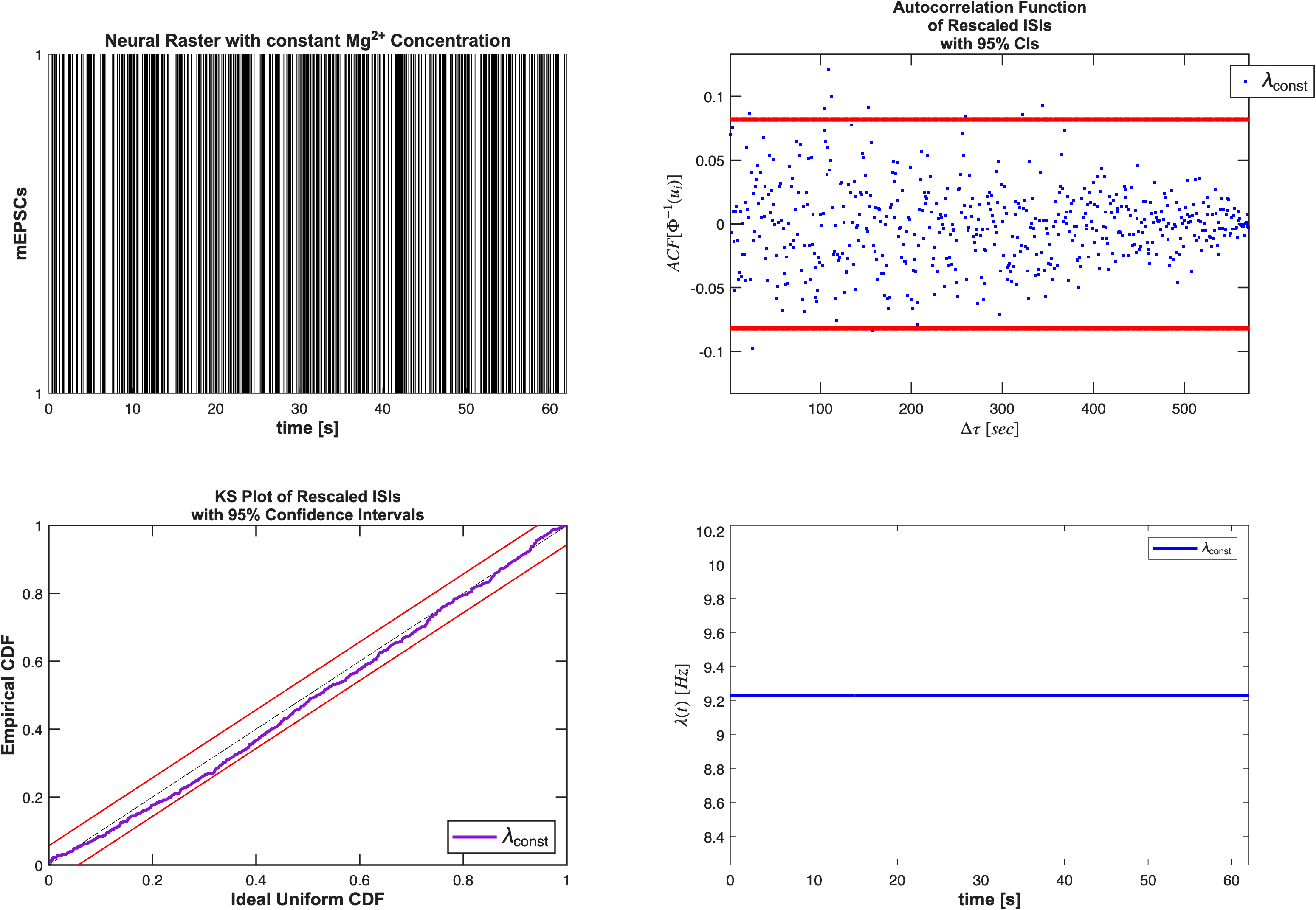
Do mEPSCs follow constant vs piecewise Poisson firing under Mg²⁺ washout?
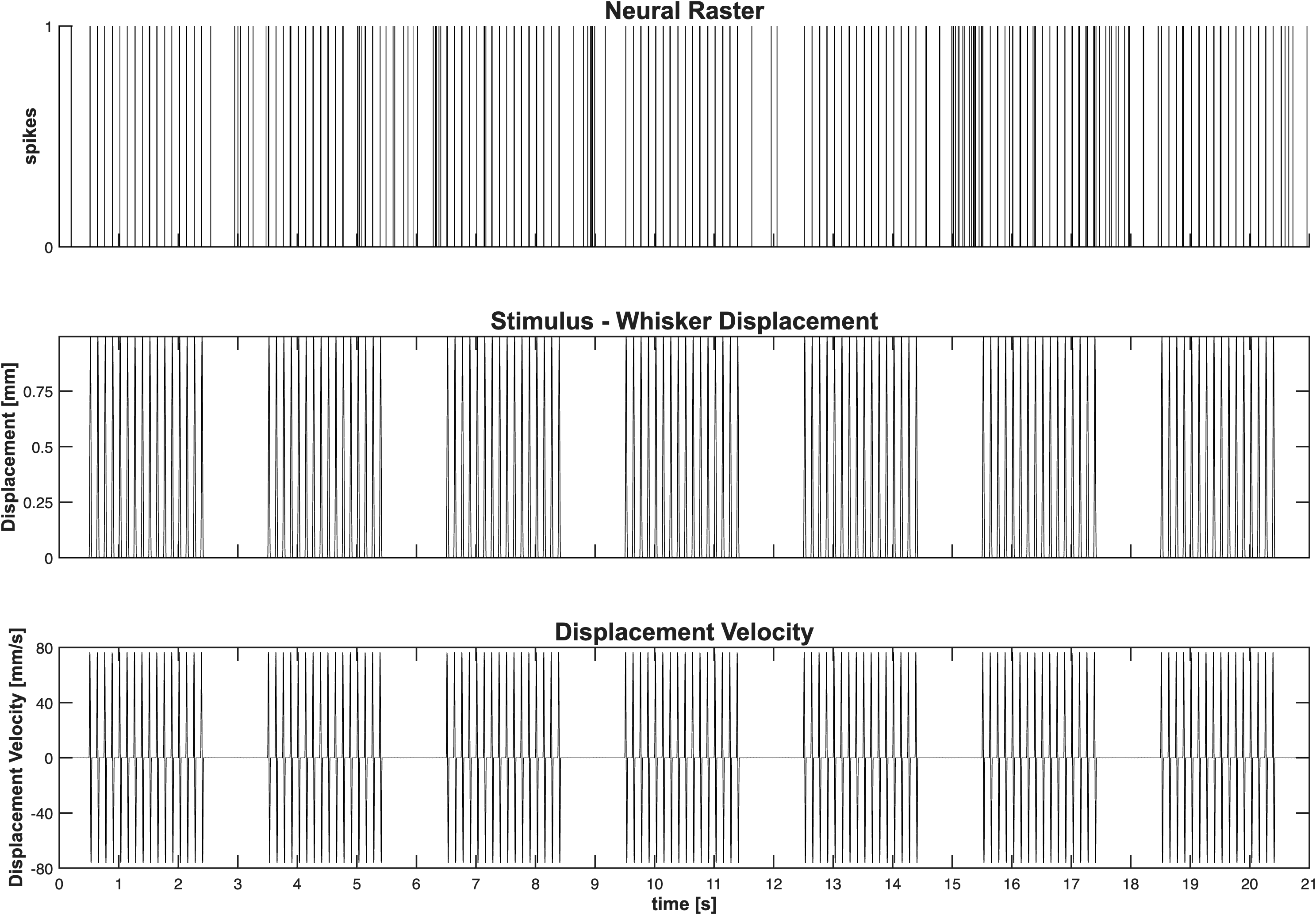
Do explicit whisker stimulus + spike history improve thalamic GLM fits?
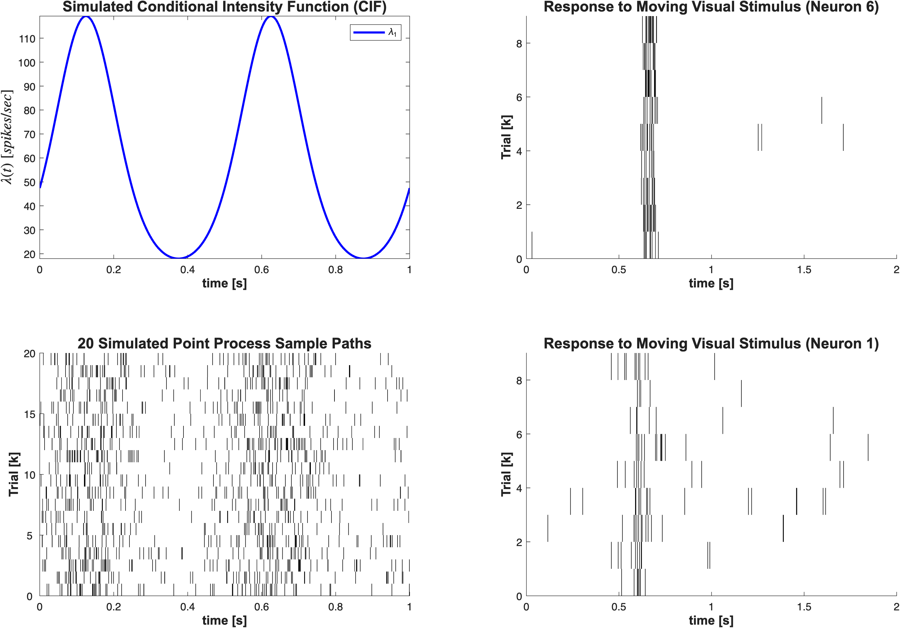
How do PSTH and SSGLM capture within-trial and across-trial dynamics?
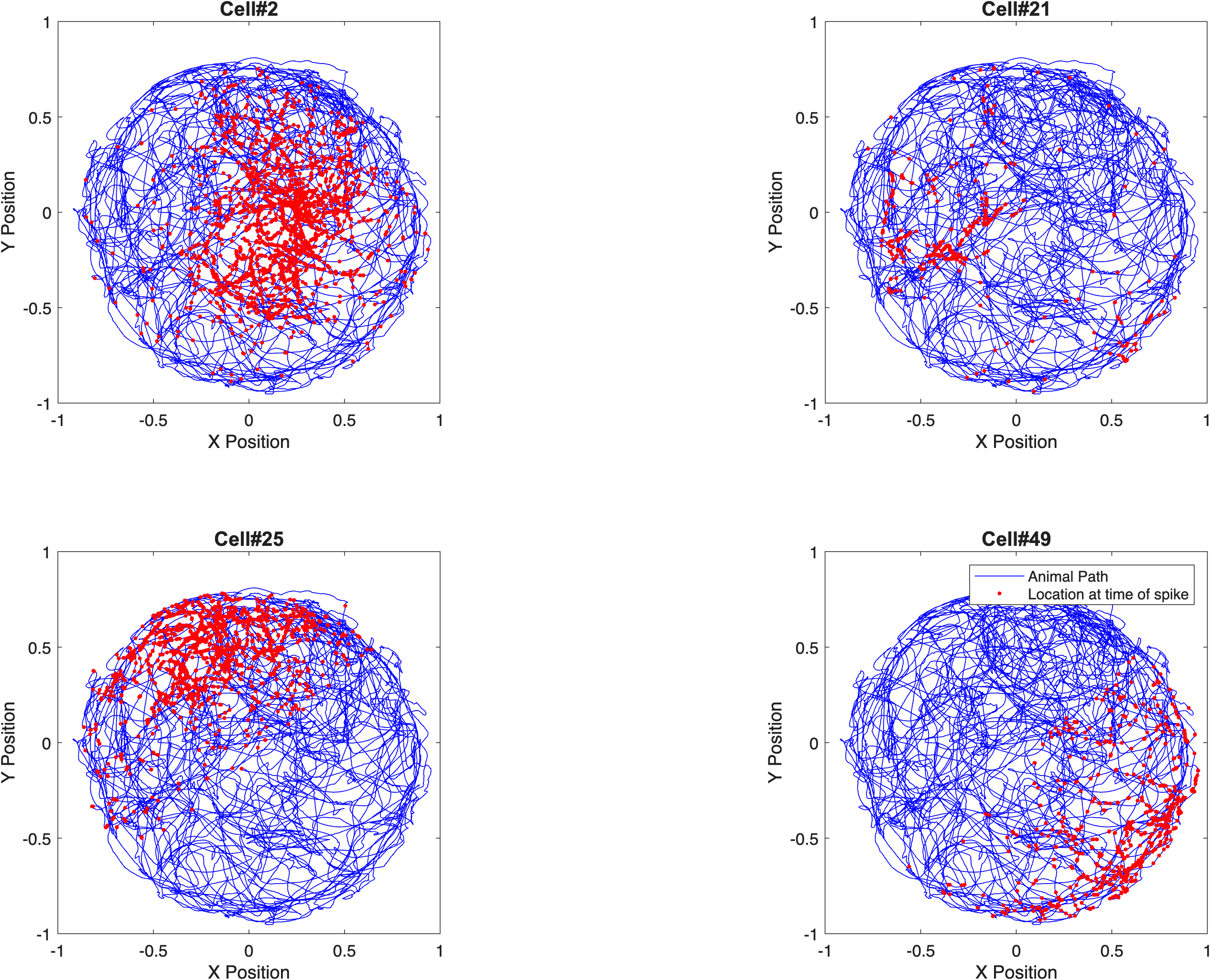
Gaussian vs Zernike receptive-field basis for hippocampal place cells?
How well do adaptive/hybrid filters decode stimulus and reach state?
Expanded gallery with all 24 figures + per-example notes: paper_examples.html.
v1.4 highlights
What landed in v1.4.0 (May 2026, two months of work):
Bernoulli LL missing
log()wrap (affects all binomial AIC/BIC/LL).KS U-clamping → inflated GOF (affects every KS plot).
DT-correction branch reachability for
λΔ > 0.4.PPAF/PPHF goal-directed time-indexing.
Multi-result λ indexing in FitResult.
+nstat/+decoding/package: 8 cluster classes.DecodingAlgorithms.m: 10860 → 1189 LOC facade.mPPCO_*→PPLFP_*(paper §4.B.7 alignment).Centralized Woodbury update.
nstat.Defaultsfor tolerances.
LinearCIF— canonical-link CIF with closed-form gradient/Hessian (drop-in forCIF, no Symbolic-Toolbox dep at eval time).History.raisedCosine(K, tMin, tMax)— Pillow 2008 log-spaced basis.Iterated-Laplace PPAF (
PPDecode_updateIterated).KS oracle integration test.
tools/run_unit_tests.sh— 20 unit tests, ~30s.tools/check_readme_figures.sh— pixel-diff drift detector for the gallery above.tools/predeploy.sh— one-command release gate.All deprecation shims warn-only; no breaking changes.
MATLAB-specific superpower — symbolic CIF derivation
What MATLAB gives you that the Python port does not (yet):
% Hand-design a conditional intensity by symbolic equation:
syms x y beta0 beta_x beta_y beta_xx beta_yy beta_xy
lambdaSymbolic = exp(beta0 + beta_x*x + beta_y*y + ...
                     beta_xx*x^2 + beta_yy*y^2 + beta_xy*x*y);

% CIF class compiles it to a fast function handle AND derives the gradient +
% Hessian w.r.t. each coefficient (used by Newton-Raphson during GLM fitting):
cif = CIF(lambdaSymbolic, {'x','y','beta0','beta_x','beta_y','beta_xx','beta_yy','beta_xy'}, ...
          {'x','y'}, 'poisson');

% The compiled handle is what Analysis.RunAnalysisForNeuron actually calls.
lambdaVal = cif.lambdaDeltaFunction(0.3, 0.5, -2, 1.1, 0.9, -0.4, -0.3, 0.2);
For canonical-link cases (Poisson + log-link, Bernoulli + logit-link) without the Symbolic-Toolbox dependency, use LinearCIF instead — it gives closed-form gradient and Hessian for the canonical-link case without symbolic round-tripping.
Where to next
The full reference docs (class definitions, every example, every algorithm).
Match 2012 paper sections to current code.
Which decoder/fitter for which problem?
SignalObj, Covariate, Trial, Analysis, FitResult, …
Same algorithms, Python idioms, opt-in extras.
Cite
If you use nSTAT in your work, please cite:
Cajigas I, Malik WQ, Brown EN. nSTAT: Open-source neural spike train analysis toolbox for Matlab. Journal of Neuroscience Methods 211(2): 245–264, Nov. 2012. DOI: 10.1016/j.jneumeth.2012.08.009 · PMID: 22981419
The 2012 paper is the canonical reference for the toolbox design and math. Subsequent changes are tracked in RELEASE_NOTES.md and % FIX: inline comments.
License: GPL v2. Code: github.com/cajigaslab/nSTAT.