Goodness-of-fit and decoding

Goal of this page. Two questions every spike-train model must answer: Does the model fit? (goodness-of-fit via time-rescaling) and Can we read out the stimulus/state from spikes? (decoding).

Glossary jumps: time-rescaling theorem · KS test / plot · population time-rescaling · encoding vs decoding · PPAF · hybrid PP filter (PPHF) · clusterless decoding

Is the model any good? The time-rescaling theorem

A low AIC means a model fits better than another model — not that it fits well. For an absolute check, nSTAT uses the time-rescaling theorem (Brown, Barbieri, Ventura, Kass & Frank 2002).

The idea is elegant. Take the fitted conditional intensity \(\lambda(t \mid H_t)\) and integrate it between consecutive spikes to get the rescaled intervals

\[ z_k \;=\; \int_{t_{k-1}}^{t_k} \lambda(u \mid H_u) \, du. \]

The theorem says: if the model is correct, the \(z_k\) are independent and exponentially distributed with rate 1 — equivalently, after the transform \(u_k = 1 - \exp(-z_k)\), they are uniform on \([0, 1]\). So you can test the model by checking whether the \(u_k\) look uniform, with a Kolmogorov–Smirnov (KS) test. nSTAT does this for you:

ks = fit.computeKSStats()
print(ks["ks_statistic"], ks["ks_pvalue"])

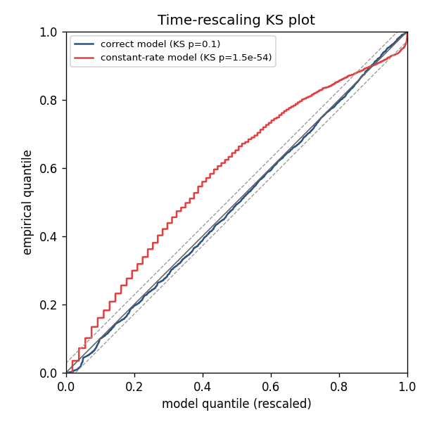
Time-rescaling KS plot comparing a correct model inside the confidence band to a constant-rate model that departs from it

The same data fit two ways. The correct model (blue) stays inside the 95% confidence band — it fits. The constant-rate model (red), which matches the mean rate but ignores the stimulus, departs far outside the band and is rejected (p ≈ 1e-54). Generated by the teaching tutorial.

Reading a KS plot. Plot the empirical CDF of the \(u_k\) against the diagonal, with 95% confidence bands. If the curve stays inside the bands, the model captures the spiking statistics. Systematic departures diagnose what is wrong:

Bowing away from the diagonal → the rate is mis-scaled.
Departures near 0 → the short-interval (refractory/history) structure is unmodeled — add or lengthen history terms.

Historical note. A bug in the MATLAB original used sampleRate instead of 1/sampleRate as the bin width, invalidating the KS test for any sampleRate ≠ 1. nSTAT-python fixes this — see the README “Code audit”.

Per-neuron is not enough: population goodness-of-fit

Each neuron can pass its own KS test while the model still misses how neurons fire together. The classic failure: model a synchronously firing pair as two independent neurons. Both per-neuron KS tests pass, yet the joint model is plainly wrong.

The multivariate (marked) time-rescaling framework of Tao, Weber, Arai & Eden (2018) catches exactly this. It rescales the population as one marked point process and applies a joint KS plus a mark χ². nSTAT implements it as a pure-NumPy core function:

from nstat import population_time_rescale

# counts_list[k]: binned spike counts for neuron k
# lam_per_bin_list[k]: the model's expected counts per bin for neuron k
res = population_time_rescale(counts_list, lam_per_bin_list, n_tau_bins=5)
print(res.ground_ks_pvalue, res.mark_chi2_pvalue)
# On a synchronous pair modeled as independent, the per-neuron KS tests pass
# but the population ground-process KS rejects at p ≈ 3e-49.

Always check both: per-neuron computeKSStats and, for population models, population_time_rescale.

Decoding: reading the stimulus/state from spikes

Goodness-of-fit asks “does the encoding model fit?” Decoding asks the inverse: given the spikes, what was the stimulus or latent state? This is how brain–machine interfaces turn motor-cortex spikes into cursor movement.

nSTAT’s workhorse is the point-process adaptive filter (PPAF) (Eden, Frank, Barbieri, Solo & Brown 2004). It is the spiking analogue of the Kalman filter: a recursive Bayesian estimator that, at each instant, predicts the state forward and then corrects the prediction using the spikes just observed, weighting by each neuron’s fitted CIF (its tuning). Because spikes are all-or-none point events rather than Gaussian measurements, the update uses the point-process likelihood instead of the Kalman gain — but the predict/correct rhythm is the same.

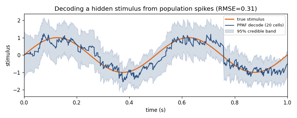
PPAF decode of a hidden sinusoidal stimulus from a 20-cell population, tracking the truth inside a 95% credible band

The PPAF reconstructs a hidden stimulus (orange) from the spikes of a 20-cell population (blue), with a 95% credible band. More cells with diverse tuning shrink the band and the error — see the runnable decoding tutorial.

Variants in nSTAT:

PPAF — continuous state (e.g. stimulus value, hand position) from a population’s spikes.
Hybrid point-process filter (PPHF) — jointly estimates a discrete mode and a continuous state (e.g. reach goal + trajectory), combining a hidden Markov model with the point-process filter.

These are exercised end-to-end in Paper Example 05.

Applying nSTAT — the clinical read-out. A decoder that returns a calibrated credible band, not just a point estimate, is what a safe clinical or BCI read-out needs. Closed-loop (adaptive) deep brain stimulation is, in control terms, exactly a decode-then-actuate loop: estimate a pathological state from the recording, then gate stimulation on it (Little et al. 2013). See Rhythmic firing and the clinical microelectrode.

Decoding without spike sorting: clusterless

Recall that spike sorting is imperfect (Harris et al. 2000) and discards information by forcing each spike into one unit. Clusterless decoding sidesteps sorting: it decodes directly from each spike’s waveform features (a “mark”), modeling the joint distribution of marks and the state. The modern state-space realization is Denovellis et al. (2021), bridged by the opt-in nstat.extras.decoding.clusterless_bridge (fit_clusterless_decoder, fit_clusterless_classifier). It is the natural descendant of nSTAT’s PPAF/PPHF for unsorted data.

Putting it together on real data: a place-cell capstone

The pieces above — encode, check, decode — come together in one walkthrough on a real recording: 49 hippocampal place cells from a rat foraging for ~24 minutes (Brown et al. 1998). We fit a place-field GLM to each cell, run the time-rescaling test, and then reconstruct the animal’s position with a Bayesian population decoder (Zhang et al. 1998) — the memoryless cousin of the PPAF, which just adds a smooth-motion prior on top of the same place-field likelihood.

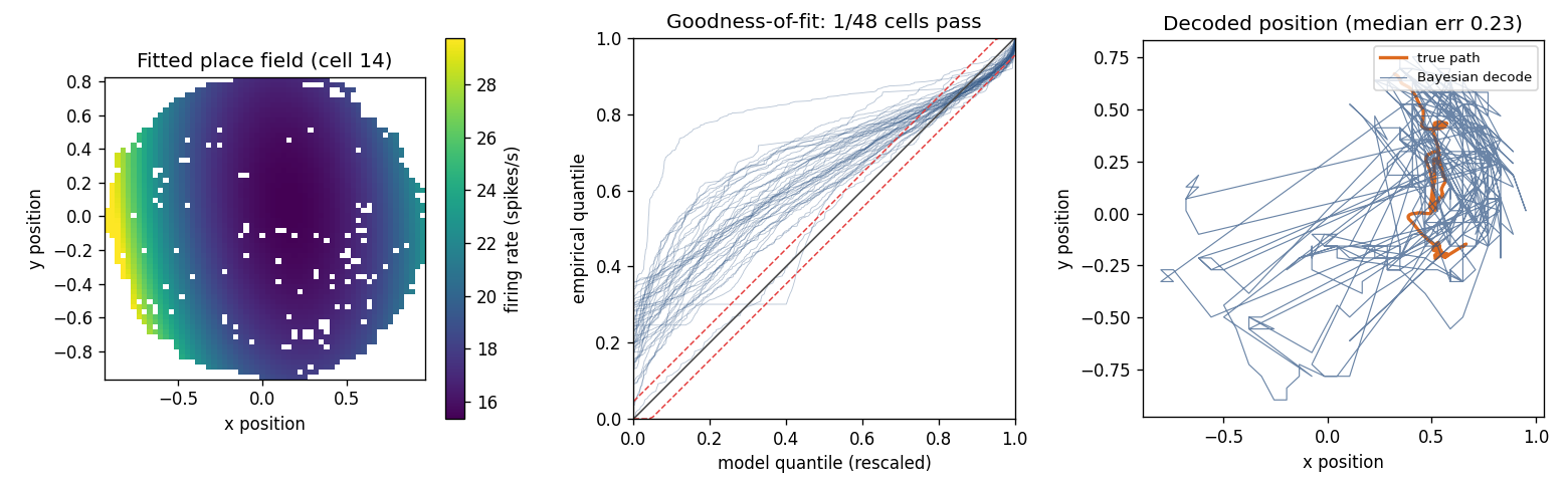
Real place-cell capstone: a fitted place field over the arena, a goodness-of-fit panel where most cells fail the KS band, and the decoded vs. true foraging trajectory

The result is a deliberately honest lesson. The place-field model decodes position several times better than chance (median error ≈ 0.23 vs. ≈ 0.84 for shuffled positions, in an arena ≈ 1.9 units wide) — yet it fails goodness-of-fit for almost every cell (1/48 pass). Useful is not the same as correct. Real place cells also carry spike history, the theta rhythm, and finer spatial structure than one Gaussian bump, and time-rescaling is what reveals the gap — pointing to the fixes: history terms (spike trains and GLMs) and a richer spatial basis (Paper Example 04’s Zernike fields). Run it with examples/tutorials/place_cell_walkthrough.py.

Check your understanding

A model has the lowest AIC of all you tried, but its KS curve leaves the confidence band. Should you trust it?
Why is decoding done from a population rather than a single neuron?
In the place-cell capstone the model decodes position well but fails the KS test. How can both be true at once?

Show answers

No. AIC only ranks models relative to each other; leaving the KS band means the model is misspecified in absolute terms. Prefer the lowest-AIC model that also passes goodness-of-fit.
A single neuron is ambiguous about the state. A population with diverse tuning jointly constrains it — decode error falls steadily as you add cells (see the decoding tutorial).
Decoding only needs the model to rank positions correctly enough to pick the right one; goodness-of-fit asks the stricter question of whether the model captures the spiking exactly. A model can be useful for the first while still being misspecified for the second — the place-field model misses spike history and theta, so it decodes well yet is rejected by KS.