Network connectivity and functional coupling
Goal of this page. Move from single neurons to interactions: how one neuron’s spikes influence another’s, how nSTAT estimates that coupling, and the classic trap of mistaking shared input for a connection.
Glossary jumps: ensemble / functional coupling · GLM · CIF · history / refractory · point process
Builds on the point-process GLM.
Neurons are not independent
A neuron’s firing depends not only on the stimulus and its own history, but on other neurons. The point-process GLM already has a slot for this — the ensemble term on the GLM page:
The term \(n_j(t - \tau)\) is neuron \(j\)’s recent spiking, and \(\eta_{ij}\) measures how it raises (\(\eta > 0\), excitation) or lowers (\(\eta < 0\), inhibition) neuron \(i\)’s firing, beyond what the shared stimulus explains. This is functional (statistical) coupling — not necessarily a direct synapse, but a directed predictive relationship (Truccolo et al. 2005).
Two ways to see coupling
1. The cross-correlogram (CCG) — model-free. Count how much more (or less) likely neuron j is to fire at each time lag relative to a neuron i spike. Excitation appears as a bump, inhibition as a trough, and the side of zero tells you the direction (who leads).
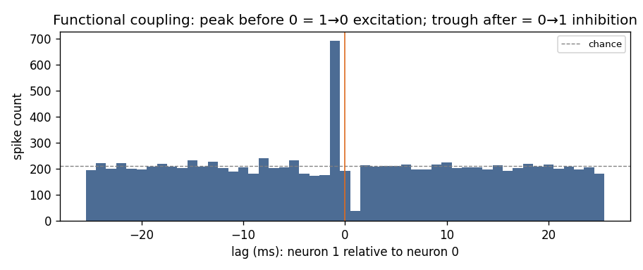
Two simulated neurons wired asymmetrically — neuron 1 excites neuron 0 (peak just before lag 0: neuron 1 leads) while neuron 0 inhibits neuron 1 (trough just after lag 0). You cannot read this directed, signed wiring from firing rates alone.
2. The coupling GLM — model-based. Fit each neuron’s firing with the other neuron’s recent spikes as a covariate; the sign and size of the fitted \(\eta\) quantify the coupling. The runnable network-coupling tutorial recovers exactly the asymmetric excite/inhibit wiring above (≈ +1.3 and −1.7, matching the simulated ±1.5).
The big trap: correlation is not connection
Two neurons that share a common input (the same stimulus, a population rhythm) will be correlated even with no direct coupling at all. A naive CCG or a coupling GLM that omits the shared drive will report a spurious connection.
The fix: include the shared stimulus (and any common covariates) in the model, so the ensemble term measures coupling over and above common input. The tutorial does this explicitly — dropping the stimulus covariate flips one of the recovered signs. This is the single most common mistake in connectivity analysis; see also Common pitfalls & FAQ.
Continuous signals: Granger causality
The same logic extends to continuous signals (e.g. LFP channels). nSTAT’s
Analysis provides ensemble Granger causality: signal X “Granger-causes”
Y if X’s past improves the prediction of Y beyond Y’s own past. It is the
continuous-signal analogue of the ensemble coupling terms above, and shares the
same common-input caveat — a third signal driving both can manufacture an
apparent causal link.
Check your understanding
A CCG shows a trough just after lag 0 (neuron j after neuron i). What coupling does that suggest, and in which direction?
Two neurons are strongly correlated. Why is that not enough to claim they are connected?
Show answers
Inhibition from i to j — neuron i’s spike makes j less likely to fire shortly after. The post-zero side indicates i leads j.
They may share a common input (stimulus or rhythm) that makes them co-vary with no direct coupling. You must condition on the shared drive before attributing correlation to a connection.
See also
Runnable tutorial (no data needed):
examples/tutorials/network_coupling.pyNotebook:
NetworkTutorial.ipynbAPI:
Analysis(Granger causality),TrialConfig(ensCovHistensemble terms),simulate_two_neuron_networkin the API reference