The LFP and spectral analysis
Goal of this page. Explain the local field potential (LFP) and the continuous-signal tools in nSTAT: multitaper spectra, spectrograms, and Kalman filtering. These apply equally to LFP, EEG, and ECoG.
Glossary jumps: LFP · EEG / ECoG · power spectral density · periodogram · multitaper method · time–bandwidth product
NW· spectrogram · Kalman filter / smoother
What the LFP is
Low-pass filter a microelectrode signal (keeping roughly 1–300 Hz) and you get the local field potential. Unlike spikes — which report individual neurons — the LFP is a population signal: it is dominated by the slower, summed synaptic and subthreshold transmembrane currents of many neurons near the electrode (Buzsáki, Anastassiou & Koch 2012).
Because it sums over a population, the LFP is the natural place to look for rhythms and coordinated activity (theta, beta, gamma bands, etc.). But interpreting it requires care: the signal at one electrode reflects contributions from a volume of tissue and is shaped by the geometry of the sources (Einevoll et al. 2013; Pesaran et al. 2018). The same machinery applies to scalp EEG and to ECoG recorded from the cortical surface — all are continuous field potentials differing mainly in scale.
In nSTAT, any such continuous signal is a SignalObj (Signal): a sampled
waveform with time base, units, and sample rate.
import numpy as np
from nstat import SignalObj

fs = 1000.0                       # Hz
t = np.arange(0, 4.0, 1 / fs)
# Toy LFP: 8 Hz theta + 40 Hz gamma + noise
x = (np.sin(2*np.pi*8*t) + 0.5*np.sin(2*np.pi*40*t)
     + 0.3*np.random.default_rng(0).standard_normal(t.size))
lfp = SignalObj(t, x, name="LFP", xlabelval="time", xunitval="s")
Why spectra, and why “multitaper”?
To ask which rhythms are present, estimate the power spectral density — how signal power is distributed across frequency. The naive estimate (squared FFT, the periodogram) is badly behaved: it is noisy (high variance that does not shrink with more data) and it leaks power between frequencies.
The multitaper method (Thomson 1982) fixes both. Instead of one window, it multiplies the data by several orthogonal Slepian (DPSS) tapers, computes a spectrum from each, and averages them. The tapers are designed to concentrate energy in a chosen frequency band, so averaging reduces variance while controlling leakage. The trade-off is a deliberate, quantified amount of spectral smoothing set by the time–bandwidth product \(NW\) (and the number of tapers \(K \approx 2 \cdot NW - 1\)). Mitra & Pesaran (1999) brought this method to neuroscience; it is the standard for LFP/EEG.
nSTAT implements it on SignalObj:
# Multitaper power spectrum (returns frequencies and power)
spec = lfp.MTMspectrum()      # peaks near 8 Hz and 40 Hz

# Other spectral estimators for comparison:
lfp.periodogram()             # single-taper (noisy) baseline
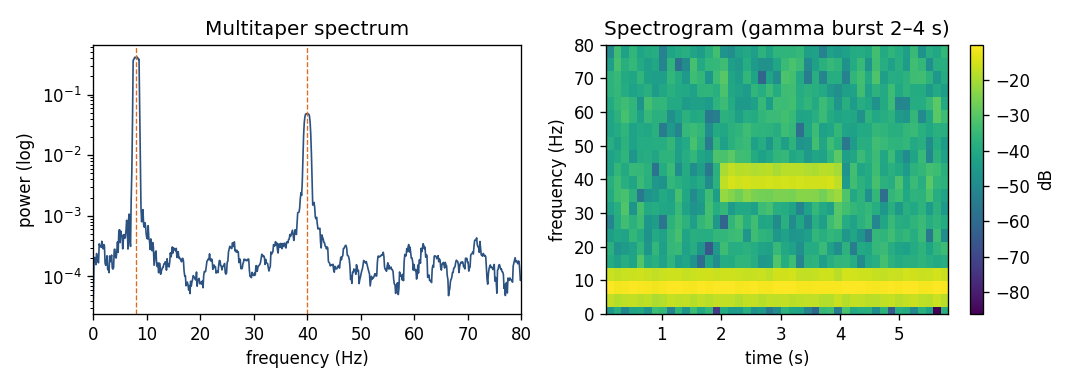
A toy LFP with 8 Hz theta throughout and a 40 Hz gamma burst from 2–4 s. Left: the multitaper spectrum cleanly resolves both peaks. Right: the spectrogram localizes the gamma burst in time — which the spectrum alone cannot.
Reading the trade-off: small NW → sharp frequency resolution but noisy;
large NW → smooth, low-variance, but blurs nearby peaks. Choose NW for the
question: separating two close rhythms needs small NW; estimating broadband
power needs large NW.
Spectrograms: how rhythms change over time
Brain rhythms are not stationary — gamma may appear only during a stimulus, theta only during movement. A spectrogram computes a multitaper spectrum in a sliding window, giving power as a function of both time and frequency:
lfp.spectrogram() # time-frequency power; see the gamma burst appear
This is the right tool for event-related spectral changes and for relating LFP rhythms to behaviour or to spiking.
Applying nSTAT — the beta biomarker for adaptive DBS. In Parkinson’s disease, beta-band (13–30 Hz) power in the subthalamic field potential tracks motor impairment and is the feedback signal for adaptive (closed-loop) deep brain stimulation (Little et al. 2013). Beta arrives in transient bursts whose duration matters more than the average (Tinkhauser et al. 2017) — exactly what a
SignalObj.spectrogramreveals that a single spectrum hides. See Rhythmic firing and the clinical microelectrode.
Other continuous-signal tools
SignalObj also provides time-domain operations useful for LFP/EEG analysis:
Cross-covariance
xcov— lagged covariance between two signals (e.g. LFP on two electrodes), for connectivity and delay estimation.Peak finding
findPeaks/findMaxima/findMinima/findGlobalPeak— detect oscillation peaks or evoked-response components.Alignment / shifting
shift,shiftMe,alignTime— line signals up to an event for averaging.Arithmetic,
power,sqrt, etc., for deriving signals.
Kalman filtering of continuous signals
When the LFP (or any continuous measurement) is a noisy observation of an
underlying latent state that evolves smoothly in time, a Kalman filter
gives the optimal (minimum-mean-square-error) estimate of that state, and the
Kalman smoother refines it using the whole recording. nSTAT provides these
in DecodingAlgorithms (e.g. kalman_filter, kalman_fixedIntervalSmoother).
For the spiking analogue — estimating a latent state from spikes rather than
a Gaussian signal — see the point-process filter on the
next page. For EM-trained linear-Gaussian
state-space models, the opt-in nstat.extras.em.dynamax_bridge wraps Dynamax.
Cross-validate your Kalman results. The
nstat.extras.validation.pykalman_bridgeruns the same filter/smoother in an independent library so you can confirm agreement — useful when learning the API.
Check your understanding
Why prefer the multitaper estimate over a raw periodogram?
You need to resolve two rhythms only a few Hz apart. Do you choose a large or a small time–bandwidth product
NW?
Show answers
The periodogram’s variance does not shrink with more data and it leaks power. Multitaper averages over orthogonal Slepian tapers, cutting variance while controlling leakage.
A small
NW— it gives sharper frequency resolution (at the cost of more variance). LargeNWover-smooths and would merge the two peaks.
See also
Runnable example: multitaper + spectrogram —
examples/readme_examples/example1_multitaper_and_spectrogram.pyNotebook:
SignalObjExamples.ipynbAPI:
SignalObj(MTMspectrum,spectrogram,periodogram,xcov,findPeaks),DecodingAlgorithmsin the API reference