Rhythmic firing and the clinical microelectrode

Goal of this page. Two ideas the other Concepts pages leave implicit. First, rhythmic (oscillatory) firing — neurons that fire to their own beat, not just to a stimulus — and how nSTAT models it with the same point-process GLM you already know. Second, the setting where this matters most concretely: a microelectrode advanced into a deep brain nucleus, the kind of recording made to guide deep brain stimulation (DBS) surgery. The same nspikeTrain, Analysis, FitResult, and SignalObj tools carry over unchanged; only the application is new.

Glossary jumps: rhythmic / oscillatory cell · tremor cell · DBS · microelectrode mapping · beta band · adaptive DBS · multitaper · spectrogram · PPAF

Rhythmic firing: when a neuron has its own beat

Most of this track models firing that is driven from outside — a stimulus, a position, a movement. But many neurons carry an intrinsic rhythm: their firing probability rises and falls periodically even with no changing stimulus. The cleanest clinical example is a tremor cell — a neuron whose firing is phase-locked to a few-hertz limb tremor — first characterized in the human subthalamic nucleus and thalamus during functional neurosurgery (Levy et al. 2000; Hutchison et al. 1998).

A rhythm is not a new kind of model — it is a covariate. If a neuron’s rate oscillates at frequency \(f\), then a pair of sine/cosine regressors at \(f\) (or a band-limited drive) enters the conditional intensity exactly like any stimulus:

\[\log \lambda(t \mid H_t) = \beta_0 + \beta_1 \sin(2\pi f t) + \beta_2 \cos(2\pi f t) + (\text{history}).\]

That is an ordinary point-process GLM (Truccolo et al. 2005), so nSTAT fits it with the machinery from the GLM page: a Covariate for the rhythmic drive, a TrialConfig, and Analysis / fit_poisson_glm. The spike-history term matters here too — rhythmicity and refractoriness both live in how a spike changes the probability of the next one.

import numpy as np
from nstat import fit_poisson_glm, population_time_rescale

# A rhythmic cell observed for 60 s at 1 kHz; tremor ~5 Hz.
dt, f = 0.001, 5.0
t = np.arange(0.0, 60.0, dt)
drive = np.sin(2 * np.pi * f * t)                 # the rhythmic covariate

# (spikes y come from your sorter; see the walkthrough script for a simulator)
# Two competing encoders: rhythm-aware vs. constant-rate.
offset = np.full(t.size, np.log(dt))
fit = fit_poisson_glm(drive[:, None], y, offset=offset, l2=1e-4)
lam_rhythm   = np.exp(fit.intercept + fit.coefficients[0] * drive + offset)
lam_constant = np.full_like(y, y.mean())

Did the rhythm model actually fit? The KS test decides

A constant-rate model and a rhythm-aware model can report the same mean rate, yet only one reproduces the timing. The time-rescaling KS test (Brown et al. 2002) is what tells them apart: the constant model leaves the confidence band, the rhythm-aware model stays inside it.

gof_rhythm   = population_time_rescale([y], [lam_rhythm])
gof_constant = population_time_rescale([y], [lam_constant])
# gof_rhythm.ground_ks_pvalue  -> large  (consistent with the model)
# gof_constant.ground_ks_pvalue -> tiny  (rejected: it gets the beat wrong)

This is the honest discipline the whole track returns to: matching the average firing rate is necessary but not sufficient — only goodness-of-fit certifies that the model captured the rhythm. The runnable clinical_microelectrode_walkthrough.py plays this contrast out end to end on a simulated tremor cell.

The clinical microelectrode: an electrode on a journey

In DBS surgery a microelectrode is lowered millimetre by millimetre toward a deep target — most often the subthalamic nucleus (STN) for Parkinson’s disease, or the globus pallidus or thalamus. The recording team listens and watches the spiking change as the tip passes through successive structures, because each nucleus has a characteristic electrophysiological signature. The STN, for instance, shows a marked rise in firing rate and burstiness on entry — a mean rate near 37 Hz with an irregular, bursty pattern, against a quieter background above (Hutchison et al. 1998). Tremor cells and movement-responsive cells appear within it; the substantia nigra below fires faster and more regularly. Everything on this page is the same nSTAT analysis you have already met, applied to that descent.

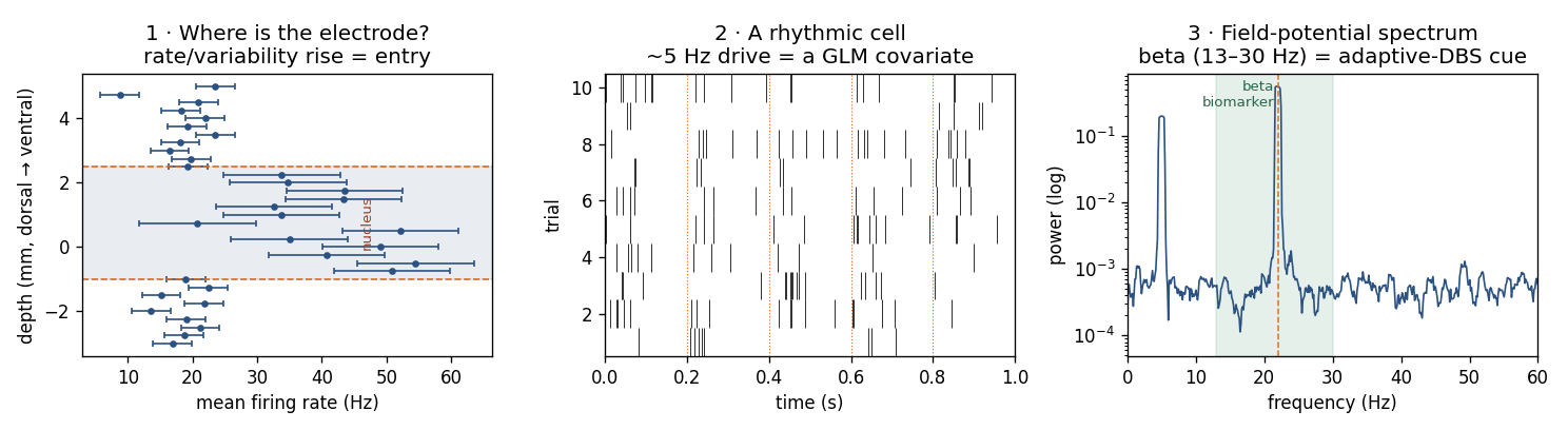
Three views of a simulated microelectrode descent: (1) mean firing rate versus depth, rising inside the nucleus; (2) a rhythmic ~5 Hz tremor cell as a spike raster; (3) the field-potential multitaper spectrum with a beta-band biomarker peak. Each maps onto a standard nSTAT object.

The three analyses this page connects, all from simulated data: (1) firing rate vs. depth — the localization cue, a latent-state problem; (2) a rhythmic cell — a point-process GLM with a periodic covariate; (3) the field-potential spectrum via SignalObj.MTMspectrum, with the beta band that guides adaptive DBS.

“Where is the electrode?” is a state-estimation problem

Tracking which structure the tip currently sits in — from a running summary of firing rate, variability, and spectral power that shifts at each boundary — is naturally a latent-state estimation problem. nSTAT supplies the estimators: a DecodingAlgorithms.kalman_filter for a continuous depth/state read out of a Gaussian summary signal, and the point-process filters below for reading state directly from spikes. The boundaries themselves (entry/exit of a nucleus) are a change-point on that latent track — the within-recording, evolving-state setting of the state-space and EM page. The spatial extent of the oscillatory territory a trajectory crosses is not a curiosity, either: the length of the dorsolateral beta-oscillatory region predicts how well DBS will work (Zaidel et al. 2010).

The beta rhythm in the field potential — a biomarker you can spectrum

Low-pass the same electrode and the local field potential carries a population rhythm of direct clinical interest: beta-band (13–30 Hz) activity in the STN scales with Parkinsonian motor impairment and is the feedback signal for adaptive (closed-loop) DBS, which stimulates only when beta is high (Little et al. 2013; Tinkhauser et al. 2017). Estimating that beta power is exactly the multitaper spectrum from the LFP page:

from nstat import SignalObj

lfp = SignalObj(t_lfp, x_lfp, name="STN field potential")
freqs, power, _ = lfp.MTMspectrum(NW=4.0)        # low-variance PSD
beta = (freqs >= 13) & (freqs <= 30)
beta_power = power[beta].sum()                    # the adaptive-DBS feature

Tinkhauser et al. showed the clinically relevant quantity is not even the average — it is the burst structure: beta arrives in transient bursts, and longer bursts track worse motor state. A SignalObj.spectrogram (sliding multitaper) is the right tool to see that time structure that a single spectrum hides.

Applying nSTAT — reading directly from spikes. When you want the latent state (tremor phase, a movement intention) from the spikes rather than the field potential, the point-process adaptive filter (DecodingAlgorithms.PPDecodeFilterLinear; Eden et al. 2004) is the spiking analogue of the Kalman filter, and it returns a calibrated credible band — the kind of honest uncertainty a clinical read-out should carry. The closed-loop DBS systems above are, in control-theoretic terms, exactly a decode-then-actuate loop (Little et al. 2013).

Where these recordings come from

nSTAT consumes spike times and sampled field potentials, not raw acquisition files. Intraoperative and research microelectrode systems write vendor formats (Spike2, Blackrock, Plexon, NEX, TDT, …); the nstat.extras.interop.neo bridge reads them through Neo and hands you the spike trains and signals to wrap in nspikeTrain / SignalObj. Detection and spike sorting happen upstream (see Microelectrode recordings); nSTAT begins once you have sorted units and an LFP.

Check your understanding

A neuron fires in time with a 5 Hz tremor, with no changing stimulus. How do you represent that rhythm in a point-process GLM, and which nSTAT object holds it?
Your rhythm-aware model and a constant-rate model report the same mean firing rate. What single test separates them, and which one passes?
You want the beta-band biomarker that drives adaptive DBS from a field potential. Which SignalObj method do you call, and why prefer it over a raw periodogram?

Show answers

Add a periodic covariate at the tremor frequency — a sin/cos pair (or a band-limited drive) — as a Covariate, exactly like any stimulus term; include a history term too, since rhythm and refractoriness both live in spike-to-spike dependence. Fit with Analysis / fit_poisson_glm.
The time-rescaling KS test (population_time_rescale / FitResult.computeKSStats). The rhythm-aware model stays inside the KS band; the constant-rate model is rejected because it matches the mean but gets the timing wrong.
SignalObj.MTMspectrum (multitaper), then sum power in 13–30 Hz. Multitaper has far lower variance and controlled leakage than the periodogram, so the beta estimate is stable; use SignalObj.spectrogram if you also need the burst time-structure.