Spike trains and point-process GLMs
Goal of this page. Explain spike trains as point processes, the conditional intensity function (CIF) that defines them, and how nSTAT fits CIFs with point-process generalized linear models (GLMs).
Glossary jumps: point process · CIF · GLM · link function · history / refractory · AIC / BIC · SSGLM
Spike trains as point processes
A point process is a probabilistic model for a series of events in time — here, spike times. Instead of predicting a continuous waveform, it predicts when discrete events happen. The complete statistical description of a point process is its conditional intensity function (CIF), written \(\lambda(t \mid H_t)\):
\(\lambda(t \mid H_t) \cdot \Delta\) ≈ the probability of a spike in the small interval \([t, t+\Delta)\), given the history \(H_t\) of everything observed up to time \(t\).
Intuitively, \(\lambda(t \mid H_t)\) is an instantaneous firing rate (in spikes/s) that is allowed to depend on the past. The dependence on history \(H_t\) is what makes the CIF powerful: it captures refractoriness, bursting, and network coupling that a plain rate \(\lambda(t)\) cannot. See Daley & Vere-Jones (2003) for the theory and Truccolo et al. (2005) for the neuroscience framing.
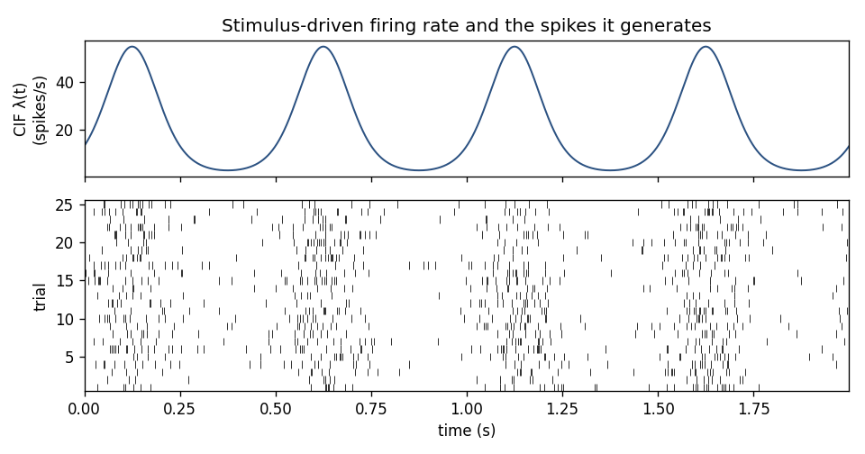
Top: a conditional intensity function \(\lambda(t)\) driven by a stimulus. Bottom: spikes simulated from it on 25 repeated trials — different every time, but denser wherever \(\lambda(t)\) is high. The point process is the bridge between the two.
Special cases worth naming:
Homogeneous Poisson: \(\lambda\) constant. Spikes are “completely random” at a fixed rate; no history dependence.
Inhomogeneous Poisson: \(\lambda(t)\) varies with time (e.g. driven by a stimulus) but still ignores history.
History-dependent (renewal and beyond): \(\lambda(t \mid H_t)\) depends on the time since the last spike(s) — the regime real neurons live in.
The point-process GLM
How do we estimate \(\lambda(t \mid H_t)\) from data? nSTAT uses a generalized linear model: model the log of the CIF as a linear combination of covariates,
Each term answers a scientific question:
Stimulus terms \(s_k(t)\) — how does an external covariate (a sensory stimulus, a movement, the animal’s position) drive firing? Often expanded in a spline or other basis so the tuning can be nonlinear.
History terms \(n(t - \tau_j)\) — how does the neuron’s own recent spiking shape its firing? Negative \(\gamma\) near zero lag captures the refractory period; positive lobes capture bursting.
Ensemble terms — does another neuron’s firing predict this one’s, beyond the shared stimulus? This is functional coupling.
Using the log link guarantees \(\lambda > 0\) (a rate can’t be negative) and makes the model multiplicative in the covariates. A central practical fact: the point-process GLM log-likelihood is concave (Paninski 2004), so fitting has a unique maximum and converges reliably — no local-minima roulette.
Fitting a GLM in nSTAT
The objects involved:
nspikeTrain/nstColl— the spike data (see Microelectrode recordings).Covariate/CovColl— the stimulus/covariate signals, sampled on a time grid.TrialConfig— which covariates, history windows, and ensemble terms to include, and the basis for each. This is your model specification.Trial— bundles spikes + covariates + events for one experiment.Analysis— runs the fit; returnsFitResultobjects.
A minimal stimulus + history fit:
import numpy as np
from nstat import (Trial, TrialConfig, ConfigColl, Covariate,
                   nstColl, nspikeTrain, Analysis)

# --- data: one unit, a 1 Hz sinusoidal stimulus over 2 s at 1 kHz ---
t = np.arange(0, 2.0, 1e-3)
stim = np.sin(2 * np.pi * 1.0 * t).reshape(-1, 1)
cov = Covariate(t, stim, name="stim", xlabelval="time", xunitval="s",
                ylabelval="amp", yunitval="a.u.", dataLabels=["stim"])

st = nspikeTrain(np.sort(np.random.default_rng(0).uniform(0, 2.0, 60)),
                 name="unit01", sampleRate=1000, minTime=0.0, maxTime=2.0)
pop = nstColl([st]); pop.setMinTime(0.0); pop.setMaxTime(2.0)
trial = Trial(pop, ev=None, covarColl=None, neighbors=None)

# --- model specification: baseline + stimulus (spline) + short history ---
cfg = TrialConfig(
    covariate_specs=[("Baseline", "constant"), ("stim", "spline")],
    sampleRate=1000,
    history_window_times=[0.001, 0.002, 0.005, 0.010],   # refractory + short
    ensCovHist=[],
)

results = Analysis.runAnalysisForAllNeurons(trial, ConfigColl([cfg]))
fit = results[0][0]
print(f"AIC = {fit.AIC:.1f}")
FitResult exposes the fitted coefficients, their confidence intervals, the
estimated CIF, and goodness-of-fit diagnostics.
Model comparison: which covariates earn their place?
More covariates always fit the training data better, so nSTAT scores models
by penalized likelihood — Akaike’s AIC and the Bayesian BIC
(fit.AIC, fit.BIC) — which trade fit against the number of parameters.
The workflow is: specify several TrialConfigs (e.g. stimulus only vs.
stimulus + history), fit all of them, and prefer the lowest AIC/BIC that
also passes goodness-of-fit (next page). A model can win on AIC and still be
wrong — always check the KS plot.
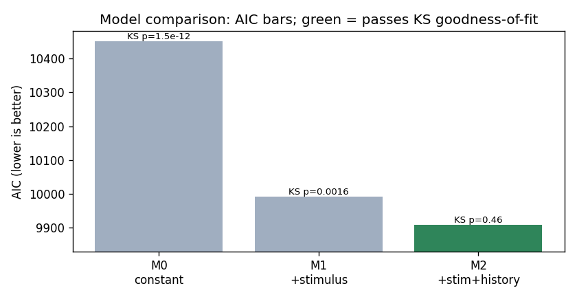
Three nested models of a neuron with a stimulus drive and a refractory period. AIC falls as terms are added, but only the full stimulus + history model passes the KS goodness-of-fit test (green) — the constant and stimulus-only models are rejected despite their lower-but-not-lowest AIC. The runnable model-comparison tutorial also reports each coefficient with a 95% confidence interval.
Across-trial dynamics: the state-space GLM (SSGLM)
The GLM above assumes the tuning is fixed. During learning, tuning changes
trial to trial. The state-space GLM treats the GLM coefficients as a
latent state that evolves across trials, estimated by an EM algorithm
(Smith & Brown 2003). In nSTAT
this is nstColl.ssglm() / ssglmFB() (forward–backward). Paper Example 03
walks through it.
Check your understanding
In words, what does \(\lambda(t \mid H_t) \cdot \Delta\) represent?
Why does the GLM model \(\log \lambda\) (a log link) rather than \(\lambda\) directly?
Show answers
The probability of a spike in the small interval \([t, t+\Delta)\), given the history \(H_t\) of past spikes and covariates.
The log link keeps the rate positive, makes covariates act multiplicatively, and yields a concave log-likelihood (Paninski 2004) so the fit has a unique optimum.
Applying nSTAT — rhythmic and tremor cells. A covariate need not be an external stimulus. A neuron with its own rhythm — for example a tremor cell locked to a few-hertz limb tremor in the human subthalamic nucleus (Levy et al. 2000) — is captured by the same GLM with a periodic covariate at the rhythm’s frequency. See Rhythmic firing and the clinical microelectrode.
See also
Runnable examples:
examples/fit_poisson_glm.py, Paper Example 02 (stimulus + history) and 03 (SSGLM).Notebooks:
AnalysisExamples.ipynb,HistoryExamples.ipynbAPI:
Analysis,TrialConfig,FitResult,CIF,fit_poisson_glmin the API referenceNext: Goodness-of-fit and decoding · Glossary · Bibliography