Population geometry: from single neurons to neural manifolds
Goal of this page. nSTAT’s models describe one neuron at a time (its conditional intensity) or pairs (functional coupling). Modern systems neuroscience adds a complementary view: treat the population’s activity as a single high-dimensional object and ask about its geometry. This page is the on-ramp — it shows the core idea with a few lines of NumPy and points to the standard tooling that takes it further.
Glossary jumps: point process · CIF · PPAF · SSGLM · ensemble / functional coupling
Why look at the population as a whole
A point-process GLM answers “what drives this neuron?” But behavior and computation are carried by populations, and the population’s activity is usually far simpler than its neuron count suggests. If you record 80 neurons, the activity does not fill all 80 dimensions — it is confined to a low-dimensional surface, a neural manifold, shaped by the variables the circuit actually represents (Gallego et al. 2017).
The simplest window onto that structure is principal component analysis (PCA): rotate the population’s activity to the axes of greatest variance and keep the first few.
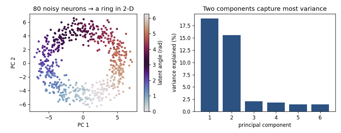
Eighty neurons, each cosine-tuned to one hidden angle (think head direction), fire as the latent variable travels around a circle. Their Poisson spike counts live in an 80-dimensional space — yet PCA reveals that the activity traces a ring in just two dimensions, with the latent angle running smoothly around it (color). The scree plot confirms two components capture most of the variance. The high-dimensional recording has a low-dimensional heart.
You can reproduce the essential computation directly from binned population counts — no new toolbox required:
import numpy as np

# counts: (T time bins) x (N neurons) spike-count matrix
Z = (counts - counts.mean(0)) / (counts.std(0) + 1e-9)   # z-score per neuron
U, S, Vt = np.linalg.svd(Z - Z.mean(0), full_matrices=False)
pcs = U[:, :2] * S[:2]                 # population trajectory in 2-D
var_explained = S**2 / np.sum(S**2)    # how flat is the manifold?
This connects straight back to nSTAT: the place-cell capstone already builds a
population spike-count matrix
(place_cell_walkthrough.py),
and decoding is the inverse question — reading the latent variable back off
the manifold.
How this relates to nSTAT’s tools
Question |
nSTAT today |
Population-geometry view |
|---|---|---|
What drives one neuron? |
point-process GLM (CIF) |
a single axis of the manifold |
How do two neurons relate? |
coupling / CCG / Granger |
local curvature of the manifold |
What is the latent state? |
PPAF / SSGLM (model-based) |
low-dim coordinates (data-driven) |
The state-space models nSTAT already implements (SSGLM, EM) and the manifold view are two routes to the same destination — a low-dimensional latent that explains many neurons. nSTAT’s route is model-based (you write down a CIF and infer the state with a filter); the manifold route is data-driven (you let variance find the axes). Each is strongest where the other is weak.
Where to learn more
nSTAT does not ship the dimensionality-reduction methods beyond this PCA sketch — that is deliberate. The standard references and tooling:
Gaussian-Process Factor Analysis (GPFA) — smooth, single-trial latent trajectories, the workhorse beyond raw PCA (Yu et al. 2009).
The dimensionality-reduction toolbox — factor analysis, demixed PCA, nonlinear embeddings; what each is for and how to choose (Cunningham & Yu 2014).
Computation through dynamics — reading the manifold as the state space of a dynamical system the circuit implements (Vyas et al. 2020).
From there the arc continues into deep-learning models of population activity — see from filters to deep learning — and the further-study page collects pointers to the topics this toolbox does not implement.
Check your understanding
You record 100 neurons but a scree plot shows the first 3 PCs capture 90% of the variance. What does that tell you about the population?
Why might a data-driven latent (PCA/GPFA) and a model-based latent (SSGLM/PPAF) disagree, and is that a problem?
Show answers
The population’s activity is low-dimensional: despite 100 neurons, the coordinated activity lives on roughly a 3-D manifold. The circuit is representing only a few underlying variables, and the neurons are correlated views of them.
They optimize different things. PCA/GPFA find the axes of greatest variance with no model of why neurons spike; SSGLM/PPAF infer the state that best explains spiking under an explicit encoding model. They can differ when high-variance activity is not the behaviorally relevant signal. It is not a problem — it is informative: agreement is reassuring, and disagreement flags that variance and task-relevance are not the same thing.
See also
State-space models and EM — the model-based route to a latent state.
Goodness-of-fit and decoding — decoding is reading the latent variable off the population.
From filters to deep learning — what comes after linear manifolds.