Uncertainty and confidence intervals

Goal of this page. Every number an analysis produces — a tuning coefficient, a firing rate, a decoded position — is an estimate from finite, noisy data. This page shows how nSTAT quantifies that uncertainty, and why an estimate without an interval is only half an answer.

Glossary jumps: GLM · CIF · link function · PPAF · SSGLM

Why a point estimate is not enough

Suppose you fit a GLM and find a stimulus coefficient of \(\beta_1 = 1.55\). Is the neuron really stimulus-driven? It depends entirely on the uncertainty: if the 95% confidence interval is \(1.55 \pm 0.10\) the effect is solid; if it is \(1.55 \pm 0.80\) you have learned almost nothing. The same estimate supports opposite conclusions depending on its interval. Reporting estimates without intervals is the single most common way a spike-train analysis overstates what the data show.

Uncertainty has one reliable cure: more (and more informative) data. As a recording lengthens, the Fisher information accumulates and the interval shrinks around the truth.

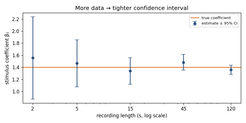
A GLM stimulus coefficient estimated from recordings of increasing length: the 95% confidence interval shrinks toward the true value as the recording grows from 2 s to 120 s

The same neuron, analyzed from progressively longer recordings. Each estimate (blue) brackets the true coefficient (orange) with its 95% interval, and the interval narrows steadily with data. With only 2 s the data are consistent with a wide range of tuning strengths; by 120 s the coefficient is pinned down.

Uncertainty in a GLM coefficient

For a point-process / Poisson GLM, the uncertainty of the fitted coefficients comes from the Fisher information — the curvature of the log-likelihood at the optimum. Sharply curved (well-identified) parameters have small standard errors; flat directions have large ones. For the Poisson GLM with design matrix \(X\) and fitted per-bin intensity \(\lambda\), the information matrix and standard errors are

\[ I(\hat\beta) \;=\; X^{\top}\,\mathrm{diag}(\lambda)\,X, \qquad \mathrm{se}(\hat\beta) \;=\; \sqrt{\mathrm{diag}\!\left(I(\hat\beta)^{-1}\right)}. \]

In Python:

import numpy as np
from nstat import fit_poisson_glm

fit = fit_poisson_glm(X, y, offset=offset)
lam = fit.predict_rate(X, offset=offset)         # fitted intensity per bin

Xaug   = np.column_stack([np.ones(len(y)), X])    # include the intercept column
fisher = Xaug.T @ (lam[:, None] * Xaug)           # Xᵀ diag(λ) X
cov    = np.linalg.pinv(fisher)                   # parameter covariance
se     = np.sqrt(np.diag(cov))                    # standard errors

# 95% confidence interval for each coefficient:
beta   = np.concatenate([[fit.intercept], fit.coefficients])
ci_low, ci_high = beta - 1.96 * se, beta + 1.96 * se

A coefficient whose CI excludes 0 is “significant” at the 5% level; one whose CI straddles 0 is not distinguishable from no effect. The worked model-comparison tutorial uses exactly this recipe to report every coefficient with its interval.

Watch the link function. These intervals are on the log-rate scale (the GLM’s linear predictor). To get an interval on the firing rate itself, transform the endpoints through \(\exp(\cdot)\) rather than adding a symmetric band to \(\exp(\beta)\) — the rate interval is asymmetric.

Uncertainty in a firing-rate curve

When you want a confidence band around a whole firing-rate estimate (a PSTH, a tuning curve, a place field), nSTAT provides DecodingAlgorithms.computeSpikeRateCIs, and computeSpikeRateDiffCIs for the difference between two conditions (e.g. stimulus vs. baseline). The bounds come back as a ConfidenceInterval object, which stores the lower/upper traces on a shared time axis and knows how to plot itself as a line pair or a shaded band.

Uncertainty in a decode

Decoding is estimation too, so a decode also carries uncertainty. The point-process adaptive filter (PPAF) propagates a posterior covariance \(W_k\) alongside the state estimate \(x_k\): the square root of its diagonal is the familiar 95% credible band around the decoded trajectory.

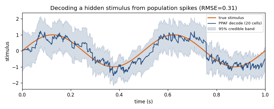
PPAF decode of a hidden sinusoidal stimulus, tracking the truth inside a 95% credible band

The decode (blue) tracks the true stimulus (orange); the shaded band is the filter’s own 95% credible interval. The band widens when spikes are sparse and tightens when the population is informative. For the across-trial SSGLM, DecodingAlgorithms.ComputeStimulusCIs builds the matching intervals (by Monte Carlo for the full cross-trial covariance, or a Gaussian z-score approximation for a smoother’s output).

Check your understanding

Two neurons both have stimulus coefficient \(\beta_1 = 0.8\), but neuron A’s 95% CI is [0.6, 1.0] and neuron B’s is [-0.3, 1.9]. Which neuron is convincingly stimulus-driven?
You halve your recording length. Roughly what happens to the width of a coefficient’s confidence interval?
Why is a 95% interval on a firing rate asymmetric even though the interval on the log-rate coefficient is symmetric?

Show answers

Neuron A. Its interval excludes 0, so the effect is reliably positive. Neuron B’s interval straddles 0 — the data are consistent with no stimulus effect at all, despite the identical point estimate.
It roughly grows by \(\sqrt{2}\) (≈ 41% wider). Standard errors scale like \(1/\sqrt{\text{information}}\), and information accumulates with data, so halving the data multiplies the interval width by about \(\sqrt{2}\).
The rate is \(\exp(\beta)\), a nonlinear transform. Pushing the symmetric endpoints \(\beta \pm 1.96 \cdot \mathrm{se}\) through \(\exp(\cdot)\) stretches the upper side more than the lower, giving an asymmetric rate interval. Transform the endpoints, never add a symmetric band to \(\exp(\beta)\).