Microelectrode recordings: spikes and the LFP
Goal of this page. Build the physical and conceptual picture of what a microelectrode records, so the rest of nSTAT (spike trains, GLMs, LFP spectra, decoding) has a concrete grounding. No prior neuroscience assumed.
Glossary jumps: microelectrode · broadband signal · LFP · action potential · single unit · multi-unit activity · spike sorting · tetrode / array · point process
What a microelectrode measures
A neuron at rest holds a voltage difference across its membrane. When it fires an action potential (“spike”), ions flow across the membrane, and those currents spread through the conductive extracellular fluid. A thin metal or silicon microelectrode placed in the tissue measures the tiny voltage these currents produce at its tip, relative to a distant reference.
The recorded voltage is a sum of contributions from many sources near the electrode. The key insight — explained thoroughly in Buzsáki, Anastassiou & Koch (2012) — is that these contributions separate cleanly by frequency:
Band (approx.) |
Name |
Physical origin |
What it tells you |
|---|---|---|---|
~300 Hz – 5 kHz (high-pass) |
Spikes / “unit activity” |
Fast action-potential currents of nearby neurons |
When individual neurons fire |
~1 – 300 Hz (low-pass) |
Local field potential (LFP) |
Slower, summed synaptic & subthreshold currents of a local population |
Coordinated population activity, rhythms |
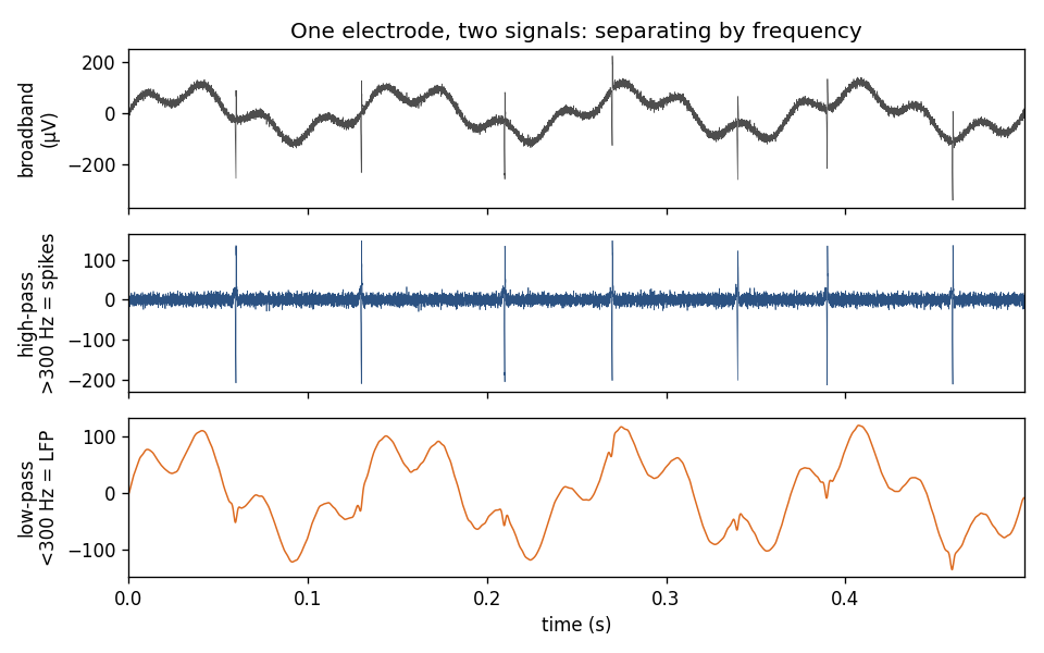
One simulated electrode signal (top) split by frequency: high-pass (>300 Hz) isolates the fast spike transients (middle); low-pass (<300 Hz) leaves the slower LFP (bottom).
So a single broadband electrode signal gives you two complementary views through two filters: high-pass it and you see spikes; low-pass it and you see the LFP. nSTAT has tools for both:
Spikes →
nspikeTrain,SpikeTrainCollection, point-process GLMs (see Spike trains and point-process GLMs).LFP →
SignalObjwith multitaper spectra, spectrograms, and Kalman filtering (see The LFP and spectral analysis).
From voltage to spike times: detection and sorting
nSTAT analyzes spike trains — lists of times at which a neuron fired — not raw voltage. Getting from the broadband trace to spike trains is a separate pre-processing pipeline:
Detection. High-pass filter the signal and mark threshold crossings; each crossing is a candidate spike waveform snippet.
Feature extraction. Reduce each snippet to a few numbers (e.g. PCA scores or wavelet coefficients).
Sorting / clustering. Group snippets by waveform shape. Because each neuron has a characteristic waveform at a given electrode, clusters correspond (approximately) to individual neurons. See Lewicki (1998) for the classic review and Quian Quiroga et al. (2004) for a popular wavelet-based method.
Single unit vs. multi-unit. A well-isolated cluster is a single unit (one putative neuron). When clusters can’t be separated, the pooled threshold crossings are multi-unit activity (MUA). Multi-electrode arrays (e.g. tetrodes) improve separation by viewing each spike from several nearby contacts.
nSTAT’s starting point. nSTAT assumes detection and sorting are already done — it consumes spike times. To go from raw acquisition files to sorted spikes, use a dedicated tool such as SpikeInterface, then bring the results into nSTAT via the interop bridges (
nstat.extras.interop.neo/.nwb/.pynapple).
Sorting is imperfect, and the errors matter. Harris et al. (2000) showed, using simultaneous intracellular ground truth, that even good tetrode sorting misassigns a non-trivial fraction of spikes. This is exactly the motivation for clusterless decoding, which skips the hard sorting step and decodes directly from spike features — see Goodness-of-fit and decoding.
Building a spike train in nSTAT
Once you have spike times (in seconds), wrap them in an nspikeTrain:
import numpy as np
from nstat import nspikeTrain

# Spike times (s) for one sorted unit, e.g. from your sorter's output.
spike_times = np.array([0.012, 0.047, 0.071, 0.130, 0.205])

st = nspikeTrain(
    spike_times,
    name="unit01",
    sampleRate=1000,   # Hz; sets the discretization grid (1 ms bins here)
    minTime=0.0,
    maxTime=0.25,
)
print(st.n_spikes, "spikes")
st.plot()   # raster tick marks
A SpikeTrainCollection (nstColl) groups units recorded together — the
natural object for population analyses and ensemble GLM terms.
from nstat import nstColl
population = nstColl([st])          # add more nspikeTrains for an ensemble
population.setMinTime(0.0)
population.setMaxTime(0.25)
Why model spike trains statistically?
A spike train looks deterministic (a neuron either fired or it didn’t), but repeated trials of the “same” stimulus produce different spike times. The productive view, formalized by Truccolo et al. (2005), is that spikes are samples from a point process whose instantaneous firing rate depends on the stimulus, the neuron’s own recent history, and the rest of the ensemble. Estimating that rate function is what nSTAT’s GLMs do, and it is the subject of the next page.
As recording counts climb into the hundreds and thousands of simultaneous neurons, principled statistical models — rather than trial-averaged tuning curves — become essential (Stevenson & Kording 2011).
Check your understanding
You have a broadband electrode trace and want the LFP. What do you do, and roughly which frequency band do you keep?
Your sorter returns a cluster you cannot cleanly separate. Is that a single unit or multi-unit activity — and can nSTAT still analyze it?
Show answers
Low-pass filter the signal, keeping roughly 1–300 Hz; the high-frequency (>300 Hz) part holds the spikes.
It is multi-unit (or unsorted) activity. nSTAT can analyze any list of spike times, but interpreting results as a single neuron requires a well-isolated unit.
See also
Runnable example: building and rastering spike trains —
examples/readme_examples/example3_nstcoll_raster_from_example2.pyNotebook:
nSpikeTrainExamples.ipynbAPI:
nspikeTrain,SpikeTrainCollection,nstCollin the API reference